LONG ANSWER QUESTIONS

Subjective Questions (With Answers)

UNIT-I

Introduction to Computer Networks

Data Communication: When we communicate, we are sharing information. This sharing can be local or remote. Between individuals, local communication usually occurs face to face, while remote communication takes place over distance.

Components:

A data communications system has five components

1. Message. The message is the information (data) to be communicated. Popular forms of information include text, numbers, pictures, audio, and video.

2. Sender. The sender is the device that sends the data message. It can be a computer, workstation, telephone handset, video camera, and so on.

3. Receiver. The receiver is the device that receives the message. It can be a computer, workstation, telephone handset, television, and so on.

4. Transmission medium. The transmission medium is the physical path by which a message travels from sender to receiver. Some examples of transmission media include twisted-pair wire, coaxial cable, fiber-optic cable, and radio waves

5. Protocol. A protocol is a set of rules that govern data communications. It represents an agreement between the communicating devices. Without a protocol, two devices may be connected but not communicating, just as a person speaking French cannot be understood by a person who speaks only Japanese.

Data Representation:

Information today comes in different forms such as text, numbers, images, audio, and video.

Text:

In data communications, text is represented as a bit pattern, a sequence of bits (Os or Is). Different sets of bit patterns have been designed to represent text symbols. Each set is called a code, and the process of representing symbols is called coding. Today, the prevalent coding system is called Unicode, which uses 32 bits to represent a symbol or character used in any language in the world. The American Standard Code for Information Interchange (ASCII), developed some decades ago in the United States, now constitutes the first 127 characters in Unicode and is also referred to as Basic Latin.

Numbers:

Numbers are also represented by bit patterns. However, a code such as ASCII is not used

to represent numbers; the number is directly converted to a binary number to simplify mathematical operations. Appendix B discusses several different numbering systems.

Images:

Images are also represented by bit patterns. In its simplest form, an image is composed of a matrix of pixels (picture elements), where each pixel is a small dot. The size of the pixel depends on the resolution. For example, an image can be divided into 1000 pixels or 10,000 pixels. In the second case, there is a better representation of the image (better resolution), but more memory is needed to store the image. After an image is divided into pixels, each pixel is assigned a bit pattern. The size and the value of the pattern depend on the image. For an image made of only black and- white dots (e.g., a chessboard), a I-bit pattern is enough to represent a pixel. If an image is not made of pure white and pure black pixels, you can increase the size of the bit pattern to include gray scale. For example, to show four levels of gray scale, you can use 2-bit patterns. A black pixel can be represented by 00, a dark gray pixel by 01, a light gray pixel by 10, and a white pixel by 11. There are several methods to represent color images. One method is called RGB, so called because each color is made of a combination of three primary colors: red, green, and blue. The intensity of each color is measured, and a bit pattern is assigned to it. Another method is called YCM, in which a color is made of a combination of three other primary colors: yellow, cyan, and magenta.

Audio:

Audio refers to the recording or broadcasting of sound or music. Audio is by nature different from text, numbers, or images. It is continuous, not discrete. Even when we use a microphone to change voice or music to an electric signal, we create a continuous signal.

Video:

Video refers to the recording or broadcasting of a picture or movie. Video can either be produced as a continuous entity (e.g., by a TV camera), or it can be a combination of images, each a discrete entity, arranged to convey the idea of motion. Again we can change video to a digital or an analog signal.

Data Flow:

Simplex:

In simplex mode, the communication is unidirectional, as on a one-way street. Only one of the two devices on a link can transmit; the other can only receive (see Figure a). Keyboards and traditional monitors are examples of simplex devices. The keyboard can only introduce input; the monitor can only accept output. The simplex mode can use the entire capacity of the channel to send data in one direction.

Half-Duplex:

In half-duplex mode, each station can both transmit and receive, but not at the same time. When one device is sending, the other can only receive, and vice versa The half-duplex mode is like a one-lane road with traffic allowed in both directions.

When cars are traveling in one direction, cars going the other way must wait. In a half-duplex transmission, the entire capacity of a channel is taken over by whichever of the two devices is transmitting at the time. Walkie-talkies and CB (citizens band) radios are both half-duplex systems.

The half-duplex mode is used in cases where there is no need for communication in both directions at the same time; the entire capacity of the channel can be utilized for each direction.

Full-Duplex:

In full-duplex both stations can transmit and receive simultaneously (see Figure c). The full-duplex mode is like a tW<D-way street with traffic flowing in both directions at the same time. In full-duplex mode, si~nals going in one direction share the capacity of the link: with signals going in the other din~c~on. This sharing can occur in two ways: Either the link must contain two physically separate t:nmsmissiIDn paths, one for sending and the other for receiving; or the capacity of the ch:arillilel is divided between signals traveling in both directions. One common example of full-duplex communication is the telephone network. When two people are communicating by a telephone line, both can talk and listen at the same time. The full-duplex mode is used when communication in both directions is required all the time. The capacity of the channel, however, must be divided between the two directions.

Network Criteria:

A network must be able to meet a certain number of criteria. The most important of these are performance, reliability, and security.

Performance:

Performance can be measured in many ways, including transit time and response time. Transit time is the amount of time required for a message to travel from one device to another. Response time is the elapsed time between an inquiry and a response. The performance of a network depends on a number of factors, including the number of users, the type of transmission medium, the capabilities of the connected hardware, and the efficiency of the software. Performance is often evaluated by two networking metrics: throughput and delay. We often need more throughputs and less delay. However, these two criteria are often contradictory. If we try to send more data to the network, we may increase throughput but we increase the delay because of traffic congestion in the network.

Reliability:

In addition to accuracy of delivery, network reliability is measured by the frequency of failure, the time it takes a link to recover from a failure, and the network's robustness in a catastrophe.

Security:

Network security issues include protecting data from unauthorized access, protecting data from damage and development, and implementing policies and procedures for recovery from breaches and data losses.

PROTOCOLS AND STANDARDS:

Protocols:

In computer networks, communication occurs between entities in different systems. An entity is anything capable of sending or receiving information. However, two entities cannot simply send bit streams to each other and expect to be understood. For communication to occur, the entities must agree on a protocol. A protocol is a set of rules that govern data communications. A protocol defines what is communicated, how it is communicated, and when it is communicated. The key elements of a protocol are syntax, semantics, and timing.

Ø  Syntax. : The term syntax refers to the structure or format of the data, meaning the order in which they are presented. For example, a simple protocol might expect the first 8 bits of data to be the address of the sender, the second 8 bits to be the address of the receiver, and the rest of the stream to be the message itself.

Ø  Semantics. : The word semantics refers to the meaning of each section of bits. How is a particular pattern to be interpreted, and what action is to be taken based on that interpretation? For example, does an address identify the route to be taken or the final destination of the message?

Ø  Timing.:  The term timing refers to two characteristics: when data should be sent and how fast they can be sent. For example, if a sender produces data at 100 Mbps but the receiver can process data at only 1 Mbps, the transmission will overload the receiver and some data will be lost.

Question No. 1

Define computer networks? Discuss various types of networks topologies in computer network. Also discuss various advantages and disadvantages of each topology.

Answer:-

“Computer network'' to mean a collection of autonomous computers interconnected by a single

technology. Two computers are said to be interconnected if they are able to exchange information. The old model of a single computer serving all of the organization's computational needs has been replaced by one in which a large number of separate but interconnected computers do the job. These systems are called computer networks.

Network topologies:

Network topology defined as the logical connection of various computers in the network.

The six basic network topologies are: bus, ring, star, tree, mesh and hybrid.

1. Bus Topology:

In bus topology all the computers are connected to a long cable called a bus. A node that wants

to send data puts the data on the bus which carries it to the destination node. In this topology any computer can data over the bus at any time. Since, the bus is shared among all the computers. When two or more computers to send data at the same time, an arbitration mechanism are needed to prevent simultaneous access to the bus.

A bus topology is easy to install but is not flexible i.e., it is difficult to add a new node to bus. In

addition to this the bus stops functioning even if a portion of the bus breaks down. It is also very difficult to isolate fault

2. Ring Topology:

In ring topology, the computers are connected in the form of a ring. Each node has exactly two

adjacent neighbors. To send data to a distant node on a ring it passes through many intermediate nodes to reach to its ultimate destination.

A ring topology is as to install and reconfigure. In this topology, fault isolation is easy because a signal that circulates all the time in a ring helps in identifying a faulty node. The data transmission takes place in only one direction. When a node fails in ring, it breaks down the whole ring. To overcome this drawback some ring topologies use dual rings. The topology is not useful to connect large number of computers.

3. Star Topology:

In star topology all the nodes are connected to a central node called a hub. A node that wants to

send some six data to some other node on the network, send data to a hub which in turn sends it the destination node. A hub plays a major role in such networks. 

Star topology is easy to install and reconfigure. If a link fails then it separates the node connected

to link from the network and the network continues to function. However, if the hub goes down, the entire network collapses.

4. Tree Topology:

Tree topology is a hierarchy of various hubs. The entire nodes are connected to one hub or the

other. There is a central hub to which only a few nodes are connected directly. The central hub, also called active hub, looks at the incoming bits and regenerates them so that they can traverse over longer distances. The secondary hubs in tree topology may be active hubs or passive hubs. The failure of a transmission line separates a node from the network.

5. Mesh Topology:

A mesh topology is also called complete topology. In this topology, each node is connected

directly to every oilier node in the network. That is if there are n nodes then there would be n(n — 1)/2 physical links in the network.

As there are dedicated links, the topology does not have congestion problems. Further it does not need a special Media Access Control (MAC) protocol to prevent simultaneous access to the transmission media since links are dedicated, not shared. The topology also provides data security. The network can continue to function even in the failure of one of the links. Fault identification is also easy. The main disadvantage of mesh topology is the complexity of the network and the cost associated with the cable length. The mesh topology is not useful for medium to large networks.

6. Hybrid Topology:

Hybrid topology is formed by connecting two or more topologies together. For example, hybrid topology can be created by using the bus, star and ring topologies

Question No. 2

What are the applications of Computer Networks?

Answer:-

1. Information:

One of the applications of computer networks is the ability to provide access to remote information.

• Pay bills; carry out transactions on bank accounts etc.

• Shop from home by inspecting the catalogs of thousands of companies available online.

• Ask the newspaper for full information about your interesting topics such as corrupt politicians, big fires, football and so on.

• Access information about health, science, art, business, cooking, sports, travel, and government and so on. All this is available on the information systems like the World Wide Web (WWW).

2. Communication:

The popular application of computer networks is electronic mail or e-mail which widely used by

millions of people to send and receive text messages. With real-time e-mail, remote users can Communicate even by see and hear each other at the same time. It is also possible to have virtual meetings called videoconference on-line among remote users.

3. Entertainment:

A huge and growing application is entertainment. It entertains people by allowing video demand, and has multiple real-time games etc.

Question No. 3

Explain about the INTERNET history?

Answer: -

The Internet has revolutionized many aspects of our daily lives. It has affected the way we do business as well as the way we spend our leisure time. Count the ways you've used the Internet recently. Perhaps you've sent electronic mail (e-mail) to a business associate, paid a utility bill, read a newspaper from a distant city, or looked up a local movie schedule-all by using the Internet. Or maybe you researched a medical topic, booked a hotel reservation, chatted with a fellow Trekkie, or comparison-shopped for a car. The Internet is a communication system that has brought a wealth of information to our fingertips and organized it for our use

A Brief History:

A network is a group of connected communicating devices such as computers and printers. An internet (note the lowercase letter i) is two or more networks that can communicate with each other. The most notable internet is called the Internet (uppercase letter I), a collaboration of more than hundreds of thousands of interconnected networks. Private individuals as well as various organizations such as government agencies, schools, research facilities, corporations, and libraries in more than 100 countries use the Internet. Millions of people are users. Yet this extraordinary communication system only came into being in 1969.

In the mid-1960s, mainframe computers in research organizations were standalone devices. Computers from different manufacturers were unable to communicate with one another. The Advanced Research Projects Agency (ARPA) in the Department of Defense (DoD) was interested in finding a way to connect computers so that the researchers they funded could share their findings, thereby reducing costs and eliminating duplication of effort.

The Internet Today:

The Internet has come a long way since the 1960s. The Internet today is not a simple hierarchical structure. It is made up of many wide- and local-area networks joined by connecting devices and switching stations. It is difficult to give an accurate representation of the Internet because it is continually changing-new networks are being added, existing networks are adding addresses, and networks of defunct companies are being removed. Today most end users who want Internet connection use the services of Internet service providers (lSPs). There are international service providers, national service providers, regional service providers, and local service providers. The Internet today is run by private companies, not the government. Figure 1.13 shows a conceptual

(not geographic) view of the Internet.

.

International Internet Service Providers:

At the top of the hierarchy are the international service providers that connect nations together.

National Internet Service Providers:

The national Internet service providers are backbone networks created and maintained by specialized companies. There are many national ISPs operating in North America; some of the most well known are SprintLink, PSINet, UUNet Technology, AGIS, and internet Mel. To provide connectivity between the end users, these backbone networks are connected by complex switching stations (normally run by a third party) called network access points (NAPs). Some national ISP networks are also connected to one another by private switching stations called peering points. These normally operate at a high data rate (up to 600 Mbps).

Regional Internet Service Providers:

Regional internet service providers or regional ISPs are smaller ISPs that are connected to one or more national ISPs. They are at the third level of the hierarchy with a smaller data rate.

Local Internet Service Providers:

Local Internet service providers provide direct service to the end users. The local ISPs can be connected to regional ISPs or directly to national ISPs. Most end users are connected to the local ISPs. Note that in this sense, a local ISP can be a company that just provides Internet services, a corporation with a network that supplies services to its own employees, or a nonprofit organization, such as a college or a university, that runs its own network. Each of these local ISPs can be connected to a regional or national service provider.

Question No. 4

What is OSI Model? Explain the functions and protocols and services of each layer?

Answer: -

The OSI Reference Model:

The OSI model (minus the physical medium) is shown in Fig. This model is based on a

proposal developed by the International Standards Organization (ISO) as a first step toward international standardization of the protocols used in the various layers (Day and Zimmermann,

1983). It was revised in 1995(Day, 1995). The model is called the ISO-OSI (Open Systems Interconnection) Reference Model because it deals with connecting open systems—that is, systems that are open for communication with other systems. The OSI model has seven layers. The principles that were applied to arrive at the seven layers can be briefly summarized as follows:

1. A layer should be created where a different abstraction is needed.

2. Each layer should perform a well-defined function.

3. The function of each layer should be chosen with an eye toward defining internationally standardized protocols.

4. The layer boundaries should be chosen to minimize the information flow across the interfaces.

5. The number of layers should be large enough that distinct functions need not be thrown together in the same layer out of necessity and small enough that the architecture does not become unwieldy

THE OSI REFERENCE MODEL

1. The Physical Layer:

              The physical layer is concerned with transmitting raw bits over a communication channel. The design issues have to do with making sure that when one side sends a 1 bit, it is received by the other side as a 1 bit, not as a 0 bit.

2. The Data Link Layer:

             The main task of the data link layer is to transform a raw transmission facility into a line that

appears free of undetected transmission errors to the network layer. It accomplishes this task by having the sender break up the input data into data frames (typically a few hundred or a few thousand bytes) and transmits the frames sequentially. If the service is reliable, the receiver confirms correct receipt of each frame by sending back an acknowledgement frame. Another issue that arises in the data link layer (and most of the higher layers as well) is how to keep a fast transmitter from drowning a slow receiver in data. Some traffic regulation mechanism is often needed to let the transmitter know how much buffer space the receiver has at the moment. Frequently, this flow regulation and the error handling are integrated.

3. The Network Layer:

           The network layer controls the operation of the subnet. A key design issue is determining how

packets are routed from source to destination. Routes can be based on static tables that are ''wired into'' the network and rarely changed. They can also be determined at the start of each conversation, for example, a terminal session (e.g., a login to a remote machine). Finally, they can be highly dynamic, being determined anew for each packet, to reflect the current network load. If too many packets are present in the subnet at the same time, they will get in one another's way, forming bottlenecks. The control of such congestion also belongs to the network layer. More generally, the quality of service provided (delay, transit time, jitter, etc.) is also a network layer issue. When a packet has to travel from one network to another to get to its destination,

many problems can arise. The addressing used by the second network may be different from the first one. The second one may not accept the packet at all because it is too large. The protocols may differ, and so on. It is up to the network layer to overcome all these problems to allow heterogeneous networks to be interconnected. In broadcast networks, the routing problem is simple, so the network layer is often thin or even nonexistent.

4. The Transport Layer:

        The basic function of the transport layer is to accept data from above, split it up into smaller units if need be, pass these to the network layer, and ensure that the pieces all arrive correctly at the other end. Furthermore, all this must be done efficiently and in a way that isolates the upper layers from the inevitable changes in the hardware technology. The transport layer also determines what type of service to provide to the session layer, and, ultimately, to the users of the network. The most popular type of transport connection is an error-free point-to-point channel that delivers messages or bytes in the order in which they were sent. However, other possible kinds of transport service are the transporting of isolated messages, with no guarantee about the order of delivery, and the broadcasting of messages to multiple destinations. The type of service is determined when the connection is established. The transport layer is a true end-to- end layer, all the way from the source to the destination. In other words, a program on the source machine carries on a conversation with a similar program on the destination machine, using the message headers and control messages. In the lower layers, the protocols are between each machine and its immediate neighbors, and not between the ultimate source and destination machines, which may be separated by many routers.

5. The Session Layer:

           The session layer allows users on different machines to establish sessions between them. Sessions offer various services, including dialog control (keeping track of whose turn it is to transmit), token management (preventing two parties from attempting the same critical operation at the same time), and synchronization (check pointing long transmissions to allow them to continue from where they were after a crash).

6. The Presentation Layer:

          The presentation layer is concerned with the syntax and semantics of the information transmitted. In order to make it possible for computers with different data representations to communicate, the data structures to be exchanged can be defined in an abstract way, along with a standard encoding to be used ''on the wire.'' The presentation layer manages these abstract data structures and allows higher-level data structures (e.g., banking records), to be defined and exchanged.

7. The Application Layer:

The application layer contains a variety of protocols that are commonly needed by users. One widely-used application protocol is HTTP (Hypertext Transfer Protocol), which is the basis for the World Wide Web. When a browser wants a Web page, it sends the name of the page it wants to the server using HTTP. The server then sends the page back. Other application protocols are used for file transfer, electronic mail, and network news.

Question No. 5

Explain the following:- a) LAN

b) MAN

c) WAN

d) ARPANET

Answer: - 
a) LAN-Local Area Networks (LAN)

           

Local area networks, generally called LANs, are privately-owned networks within a single building or campus of up to a few kilometers in size. They are widely used to connect personal computers and workstations in company offices and factories to share resources (e.g., printers) and exchange information. LANs are distinguished from other kinds of networks by three characteristics:

(1) Their size,

(2) Their transmission technology, and

(3) Their topology.

LANs are restricted in size, which means that the worst-case transmission time is bounded and known in advance. Knowing this bound makes it possible to use certain kinds of designs that would not otherwise be possible. It also simplifies network management. LANs may use a transmission technology consisting of a cable to which all the machines are attached, like the telephone company party lines once used in rural areas. Traditional LANs run at speeds of 10 Mbps to 100 Mbps, have low delay (microseconds or nanoseconds), and make very few errors

Newer LANs operate at up to 10 Gbps various topologies are possible for broadcast LANs. Figure shows two of them. In a bus (i.e., a linear cable) network, at any instant at most one machine is the master and is allowed to transmit. All other machines are required to refrain from sending. An arbitration mechanism is needed to resolve conflicts when two or more machines want to transmit simultaneously. The arbitration mechanism may be centralized or distributed. IEEE 802.3, popularly called Ethernet, for example, is a bus-based broadcast network with decentralized control, usually operating at 10 Mbps to 10 Gbps. Computers on an Ethernet can transmit whenever they want to; if two or more packets collide, each computer just waits a random time and tries again later.

A second type of broadcast system is the ring. In a ring, each bit propagates around on its own, not waiting for the rest of the packet to which it belongs. Typically, each bit circumnavigates the entire ring in the time it takes to transmit a few bits, often before the complete packet has even been transmitted. As with all other broadcast systems, some rule is needed for arbitrating simultaneous accesses to the ring. Various methods, such as having the machines take turns, are in use. IEEE 802.5 (the IBM token ring), is a ring-based LAN operating at 4 and 16 Mbps. FDDI is another example of a ring network.

b) Metropolitan Area Network:

A metropolitan area network, or MAN, covers a city. The best-known example of a MAN is the

Cable television network available in many cities. This system grew from earlier community antenna systems used in areas with poor over-the-air television reception. In these early systems, a large antenna was placed on top of a nearby hill and signal was then piped to the subscribers' houses.

At first, these were locally-designed, ad hoc systems. Then companies began jumping into the business, getting contracts from city governments to wire up an entire city. The next step was television programming and even entire channels designed for cable only. Often these channels were highly specialized, such as all news, all sports, all cooking, all gardening, and so on. But from their inception until the late 1990s, they were intended for television reception only.

To a first approximation, a MAN might look something like the system shown in Fig.2. In this figure both television signals and Internet are fed into the centralized head end for subsequent distribution to people's homes.

Cable television is not the only MAN. Recent developments in high-speed wireless Internet access resulted in another MAN, which has been standardized as IEEE 802.16. A MAN is implemented by a standard called DQDB (Distributed Queue Dual Bus) or IEEE 802.16. DQDB has two unidirectional buses (or cables) to which all the computers are attached.

c) Wide Area Network:

               A wide area network, or WAN, spans a large geographical area, often a country or continent. It contains a collection of machines intended for running user (i.e., application) programs. These machines are called as hosts. The hosts are connected by a communication subnet, or just subnet for short. The hosts are owned by the customers (e.g., people's personal computers), whereas the communication subnet is typically owned and operated by a telephone company or Internet service provider. The job of the subnet is to carry messages from host to host, just as the telephone system carries words from speaker to listener. Separation of the pure communication aspects of the network (the subnet) from the application aspects (the hosts), greatly simplifies the complete network design.

In most wide area networks, the subnet consists of two distinct components: transmission lines and switching elements. Transmission lines move bits between machines. They can be made of copper wire, optical fiber, or even radio links. In most WANs, the network contains numerous transmission lines, each one connecting a pair of routers. If two routers that do not share a transmission line wish to communicate, they must do this indirectly, via other routers. When a packet is sent from one router to another via one or more intermediate routers, the packet is received at each intermediate router in its entirety, stored there until the required output line is free, and then forwarded. A subnet organized according to this principle is called a store-and- forward or packet-switched subnet. Nearly all wide area networks (except those using satellites) have store-and-forward subnets. When the packets are small and all the same size, they are often called cells.

           The principle of a packet-switched WAN is so important. Generally, when a process on some host has a message to be sent to a process on some other host, the sending host first cuts the message into packets, each one bearing its number in the sequence. These packets are then injected into the network one at a time in quick succession. The packets are transported individually over the network and deposited at the receiving host, where they are reassembled into the original message and delivered to the receiving process. A stream of packets resulting from some initial message is illustrated. In this figure, all the packets follow the route ACE, rather than ABDE or ACDE. In some networks all packets from a given message must follow the same route; in others each packed is routed separately. Of course, if ACE is the best route, all packets may be sent along it, even if each packet is individually routed.

Not all WANs are packet switched. A second possibility for a WAN is a satellite system. Each router has an antenna through which it can send and receive. All routers can hear the output from the satellite, and in some cases they can also hear the upward transmissions of their fellow routers to the satellite as well. Sometimes the routers are connected to a substantial point-to-point subnet, with only some of them having a satellite antenna. Satellite networks are inherently broadcast and are most useful when the broadcast property is important.

d) ARPANET:

            The subnet would consist of minicomputers called IMPs (Interface Message Processors) Connected by 56-kbps transmission lines. For high reliability, each IMP would be connected to at least two other IMPs. The subnet was to be a datagram subnet, so if some lines and IMPs were destroyed, messages could be automatically rerouted along alternative paths.

           Each node of the network was to consist of an IMP and a host, in the same room, connected by a short wire. A host could send messages of up to 8063 bits to its IMP, which would then break these up into packets of at most 1008 bits and forward them independently toward the destination. Each packet was received in its entirety before being forwarded, so the subnet was the first electronic store-and-forward packet-switching network.

Each node of the network was to consist of an IMP and a host, in the same room, connected by a

short wire. A host could send messages of up to 8063 bits to its IMP, which would then break these up into packets of at most 1008 bits and forward them independently toward the destination. Each packet was received in its entirety before being forwarded, so the subnet was the first electronic store-and-forward packet-switching network.

ARPA then put out a tender for building the subnet. Twelve companies bid for it. After evaluating all the proposals, ARPA selected BBN, a consulting firm in Cambridge, Massachusetts, and in December 1968, awarded it a contract to build the subnet and write the subnet software. BBN chose to use specially modified Honeywell DDP-316 minicomputers with

12K 16-bit words of core memory as the IMPs. The IMPs did not have disks, since moving parts were considered unreliable. The IMPs were interconnected by 56-kbps lines leased from telephone companies. Although 56 kbps is now the choice of teenagers who cannot afford ADSL or cable, it was then the best money could buy.

The software was split into two parts: subnet and host. The subnet software consisted of the IMP end of the host-IMP connection, the IMP-IMP protocol, and a source IMP to destination IMP protocol designed to improve reliability. The original ARPANET design is shown in Fig.10. Outside the subnet, software was also needed, namely, the host end of the host-IMP connection, the host-host protocol, and the application software. It soon became clear that BBN felt that when it had accepted a message on a host-IMP wire and placed it on the host-IMP wire at the destination, its job was done.

Question No. 6

What is TCP/IP Model? Explain the functions and protocols and services of each layer? Compare it with OSI Model. 

Answer: -

The TCP/IP MODEL:-

The TCP/IP reference model was developed prior to OSI model. The major design goals of this

model were,

1. To connect multiple networks together so that they appear as a single network.

2. To survive after partial subnet hardware failures.

3. To provide a flexible architecture.

Unlike OSI reference model, TCP/IP reference model has only 4 layers. They are,

1. Host-to-Network Layer

2. Internet Layer

3. Transport Layer

4. Application Layer

1. Host-to-Network Layer:

The TCP/IP reference model does not really say much about what happens here, except to point

out that the host has to connect to the network using some protocol so it can send IP packets to it. This protocol is not defined and varies from host to host and network to network.

2. Internet Layer:

This layer, called the internet layer, is the linchpin that holds the whole architecture together. Its

job is to permit hosts to inject packets into any network and have they travel independently to the destination (potentially on a different network). They may even arrive in a different order than they were sent, in which case it is the job of higher layers to rearrange them, if in-order delivery is desired. Note that ''internet'' is used here in a generic sense, even though this layer is present in the Internet.

The internet layer defines an official packet format and protocol called IP (Internet Protocol). The job of the internet layer is to deliver IP packets where they are supposed to go. Packet routing is clearly the major issue here, as is avoiding congestion. For these reasons, it is reasonable to say that the TCP/IP internet layer is similar in functionality to the OSI network layer.

3. The Transport Layer:

The layer above the internet layer in the TCP/IP model is now usually called the transport layer.

It is designed to allow peer entities on the source and destination hosts to carry on a conversation, just as in the OSI transport layer. Two end-to-end transport protocols have been defined here. The first one, TCP (Transmission Control Protocol), is a reliable connection- oriented protocol that allows a byte stream originating on one machine to be delivered without error on any other machine in the internet. It fragments the incoming byte stream into discrete messages and passes each one on to the internet layer. At the destination, the receiving TCP process reassembles the received messages into the output stream. TCP also handles flow control to make sure a fast sender cannot swamp a slow receiver with more messages than it can handle.

The second protocol in this layer, UDP (User Datagram Protocol), is an unreliable, connectionless protocol for applications that do not want TCP's sequencing or flow control and wish to provide their own. It is also widely used for one-shot, client-server-type request-reply queries and applications in which prompt delivery is more important than accurate delivery, such as transmitting speech or video. Since the model was developed, IP has been implemented on many other networks.

4. The Application Layer:

The TCP/IP model does not have session or presentation layers. On top of the transport layer is

the application layer. It contains all the higher-level protocols. The early ones included virtual terminal (TELNET), file transfer (FTP), and electronic mail (SMTP), as shown in Fig.6.2. The virtual terminal protocol allows a user on one machine to log onto a distant machine and work there. The file transfer protocol provides a way to move data efficiently from one machine to another. Electronic mail was originally just a kind of file transfer, but later a specialized protocol (SMTP) was developed for it. Many other protocols have been added to these over the years: the Domain Name System (DNS) for mapping host names onto their network addresses, NNTP, the protocol for moving USENET news articles around, and HTTP, the protocol for fetching pages on the World Wide Web, and many others.

Comparison of the OSI and TCP/IP Reference Models:

The OSI and TCP/IP reference models have much in common. Both are based on the concept of

a stack of independent protocols. Also, the functionality of the layers is roughly similar. For example, in both models the layers up through and including the transport layer are there to provide an end-to-end, network-independent transport service to processes wishing to communicate. These layers form the transport provider. Again in both models, the layers above transport are application-oriented users of the transport service. Despite these fundamental similarities, the two models also have many differences.

Three concepts are central to the OSI model:

1. Services.

2. Interfaces.

3. Protocols.

Probably the biggest contribution of the OSI model is to make the distinction between these three concepts explicit. Each layer performs some services for the layer above it. The service definition tells what the layer does, not how entities above it access it or how the layer works. It defines the layer's semantics. A layer's interface tells the processes above it how to access it. It specifies what the parameters are and what results to expect. It, too, says nothing about how the layer works inside.

Finally, the peer protocols used in a layer are the layer's own business. It can use any protocols it wants to, as long as it gets the job done (i.e., provides the offered services). It can also change them at will without affecting software in higher layers. The TCP/IP model did not originally clearly distinguish between service, interface, and protocol, although people have tried to retrofit it after the fact to make it more OSI-like. For example, the only real services offered by the internet layer are SEND IP PACKET and RECEIVE IP PACKET.

As a consequence, the protocols in the OSI model are better hidden than in the TCP/IP model and can be replaced relatively easily as the technology changes. Being able to make such changes is one of the main purposes of having layered protocols in the first place. The OSI reference model was devised before the corresponding protocols were invented.

This ordering means that the model was not biased toward one particular set of protocols, a fact that made it quite general. The downside of this ordering is that the designers did not have much experience with the subject and did not have a good idea of which functionality to put in which layer.

Another difference is in the area of connectionless versus connection-oriented communication. The OSI model supports both connectionless and connection-oriented communication in the network layer, but only connection-oriented communication in the transport layer, where it counts (because the transport service is visible to the users). The TCP/IP model has only one mode in the network layer (connectionless) but supports both modes in the transport layer, giving the users a choice. This choice is especially important for simple request-response protocols.

Question No. 7

Explain about the different types of transmission Medias in computer networks?

Answer: - 

Network media is the actual path over which an electrical signal travels as it moves from one       component to another. There are some common types of network media, including twisted-pair Cable, coaxial cable, fiber-optic cable, and wireless.

GUIDED MEDIA

Guided media, which are those that provide a conduit from one device to another, include twisted-pair cable, coaxial cable, and fiber-optic cable. A signal traveling along any of these media is directed and contained by the physical limits of the medium. Twisted-pair and coaxial cable use metallic (copper) conductors that accept and transport signals in the form of electric current. Optical fiber is a cable that accepts and transports signals in the form of light.

Twisted-Pair Cable

A twisted pair consists of two conductors (normally copper), each with its own plastic insulation, twisted together, as shown in following figure.

One of the wires is used to carry signals to the receiver, and the other is used only as a ground reference. The receiver uses the difference between the two.In addition to the signal sent by the sender on one of the wires, interference (noise) and crosstalk may affect both wires and create unwanted signals. If the two wires are parallel, the effect of these unwanted signals is not the same in both wires because they are at different locations relative to the noise or crosstalk sources (e.g., one is closer and the other is farther). This results in a difference at the receiver. By twisting the pairs, a balance is maintained. For example, suppose in one twist, one wire is closer to the noise source and the other is farther; in the next twist, the reverse is true. Twisting makes it probable that both wires are equally affected by external influences (noise or crosstalk). This means that the receiver, which calculates the difference between the two, receives no unwanted signals. The unwanted signals are mostly canceled out. From the above discussion, it is clear that the number of twists per unit of length (e.g., inch) has some effect on the quality of the cable.

Unshielded Versus Shielded Twisted-Pair Cable

The most common twisted-pair cable used in communications is referred to as unshielded twisted-pair (UTP). IBM has also produced a version of twisted-pair cable for its use, called shielded twisted-pair (STP). STP cable has a metal foil or braided mesh covering that encases each pair of insulated conductors. Although metal casing improves the quality of cable by preventing the penetration of noise or crosstalk, it is bulkier and more expensive. Below figure

ii.Shielded Twisted-Pair Cable

Ø  Shielded twisted-pair (STP) cable combines the techniques of shielding, cancellation, and wire twisting. Each pair of wires is wrapped in a metallic foil .The four pairs of wires then are wrapped in an overall metallic braid or foil, usually 150-ohm cable. STP usually is installed with STP data connector, which is created especially for the STP cable. However, STP cabling also can use the same RJ connectors that UTP uses.

Ø  Although STP prevents interference better than UTP, it is more expensive and difficult to install. In addition, the metallic shielding must be grounded at both ends. If it is improperly grounded, the shield acts like an antenna and picks up unwanted signals. Because of its cost and difficulty with termination, STP is rarely used in Ethernet networks. STP is primarily used in Europe.

The following summarizes the features of STP cable:

Ø  Speed and throughput—10 to 100 Mbps

Ø  Average cost per node—Moderately expensive

Ø  Media and connector size—Medium to large

Ø  Maximum cable length—100 m (short)

Coaxial Cable

Ø  Coaxial cable consists of a hollow outer cylindrical conductor that surrounds a single inner wire made of two conducting elements. One of these elements, located in the center of the cable, is a copper conductor. Surrounding the copper conductor is a layer of flexible insulation. Over this insulating material is a woven copper braid or metallic foil that acts both as the second wire in the circuit and as a shield for the inner conductor. This second layer, or shield, can help reduce the amount of outside interference. Covering this shield is the cable jacket.

Ø  Coaxial cable supports 10 to 100 Mbps and is relatively inexpensive, although it is more costly than UTP on a per-unit length. However, coaxial cable can be cheaper for a physical bus topology because less cable will be needed. Coaxial cable can be cabled over longer distances than twisted-pair cable. For example, Ethernet can run approximately 100 meters (328 feet) using twisted-pair cabling. Using coaxial cable increases this distance to 500m (1640.4 feet).

Ø  For LANs, coaxial cable offers several advantages. It can be run with fewer boosts from repeaters for longer distances between network nodes than either STP or UTP cable. Repeaters regenerate the signals in a network so that they can cover greater distances. Coaxial cable is less expensive than fiber-optic cable, and the technology is well known; it has been used for many years for all types of data communication.

Ø  When working with cable, you need to consider its size. As the thickness, or diameter, of the cable increases, so does the difficulty in working with it. Many times cable must be pulled through existing conduits and troughs that are limited in size. Coaxial cable comes in a variety of sizes. The largest diameter (1 centimeter [cm]) was specified for use as Ethernet backbone cable because historically it had greater transmission length and noise-rejection characteristics. In the past, coaxial cable with an outside diameter of only 0.35 cm (sometimes referred to as Thinnet) was used in Ethernet network

The following summarizes the features of coaxial cables:

Ø  Speed and throughput—10 to 100 Mbps

Ø  Average cost per node—Inexpensive

Ø  Media and connector size—Medium

Maximum cable length—500 m (medium)

Fiber-Optic Cable

A fiber-optic cable is made of glass or plastic and transmits signals in the form of light. To understand optical fiber, we first need to explore several aspects of the nature of light. Light travels in a straight line as long as it is moving through a single uniform substance. If a ray of

light traveling through one substance suddenly enters another substance (of a different density), the ray changes direction. Below figure shows how a ray of light changes direction when going from a denser to a less dense substance. As the figure shows, if the angle of incidence I (the angle the ray makes with the line perpendicular to the interface between the two substances) is less than the critical angle, the ray refracts and moves closer to the surface. If the angle of incidence is equal to the critical angle, the light bends along the interface. If the angle is greater than the critical angle, the ray reflects (makes a turn) and travels again in the denser

substance . Note that the critical angle is a property of the substance, and its value differs from one substance to another. Optical fibers use reflection to guide light through a channel. A glass or plastic core is surrounded by a cladding of less dense glass or plastic. The difference in density of the two materials must be such that a beam of light moving through the core is reflected off the cladding instead of being refracted into it. See below figure.

UNGUIDED MEDIA: WIRELESS

Unguided medium transport electromagnetic waves without using a physical conductor. This type of communication is often referred to as wireless communication. Signals are normally broadcast through free space and thus are available to anyone who has a device capable of receiving them. Below figure 7.17 shows the part of the electromagnetic spectrum, ranging from 3 kHz to 900 THz, used for wireless communication. Unguided signals can travel from the source to the destination in several ways: ground propagation, sky propagation, and line-of-sight propagation, as shown in below figure.

In ground propagation, radio waves travel through the lowest portion of the atmosphere, hugging the earth. These low-frequency signals emanate in all directions from the transmitting antenna and follow the curvature of the planet. Distance depends on the amount of power in the signal: The greater the power, the greater the distance. In sky propagation, higher-frequency radio waves radiate upward into the ionosphere (the layer of atmosphere where particles exist as ions) where they are reflected back to earth. This type of transmission allows for greater distances with lower output power. In line-of-sight propagation, very high-frequency signals are transmitted in straight lines directly from antenna to antenna.

The section of the electromagnetic spectrum defined as radio waves and microwaves is divided into eight ranges, called bands, each regulated by government authorities. These bands are rated from very low frequency (VLF) to extremely high frequency (EHF). Below table lists these bands, their ranges, propagation methods, and some applications

Radio Waves

Although there is no clear-cut demarcation between radio waves and microwaves, electromagnetic waves ranging in frequencies between 3 kHz and 1 GHz are normally called radio waves; waves ranging in frequencies between I and 300 GHz are called microwaves. However, the behavior of the waves, rather than the frequencies, is a better criterion for classification. Radio waves, for the most part, are omnidirectional. When an antenna transmits radio waves, they are propagated in all directions. This means that the sending and receiving antennas do not have to be aligned. A sending antenna sends waves that can be received by any receiving antenna. The omnidirectional property has a disadvantage, too. The radio waves transmitted by one antenna are susceptible to interference by another antenna that may send signals using the same frequency or band. Radio waves, particularly those waves that propagate in the sky mode, can travel long distances. This makes radio waves a good candidate for long- distance broadcasting such as AM radio.

Omni directional Antenna

Radio waves use omni directional antennas that send out signals in all directions. Based on the wavelength, strength, and the purpose of transmission, we can have several types of antennas. Below Figure shows an omni directional antenna.

Microwaves

Electromagnetic waves having frequencies between 1 and 300 GHz are called microwaves. Microwaves are unidirectional. When an antenna transmits microwaves, they can be narrowly focused. This means that the sending and receiving antennas need to be aligned. The unidirectional property has an obvious advantage. A pair of antennas can be aligned without interfering with another pair of aligned antennas.

The following describes some characteristics of microwave propagation:

 Microwave propagation is line-of-sight. Since the towers with the mounted antennas need to be in direct sight of each other, towers that are far apart need to be very tall. The curvature of the earth as well as other blocking obstacles does not allow two short towers to communicate by using microwaves. Repeaters are often needed for long distance communication.

 Very high-frequency microwaves cannot penetrate walls. This characteristic can be a disadvantage if receivers are inside buildings.

 The microwave band is relatively wide, almost 299 GHz. Therefore wider subbands can be assigned, and a high data rate is possible.

 Use of certain portions of the band requires permission from authorities.

Unidirectional Antenna

Microwaves need unidirectional antennas that send out signals in one direction. Two types of antennas are used for microwave communications: the parabolic dish and the horn .

A parabolic dish antenna is based on the geometry of a parabola: Every line parallel to the line of symmetry (line of sight) reflects off the curve at angles such that all the lines intersect in a common point called the focus. The parabolic dish works as a funnel, catching a wide range of waves and directing them to a common point. In this way, more of the signal is recovered than would be possible with a single-point receiver.

Outgoing transmissions are broadcast through a horn aimed at the dish. The microwaves

hit the dish and are deflected outward in a reversal of the receipt path. A horn antenna looks like a gigantic scoop. Outgoing transmissions are broadcast up a stem (resembling a handle) and deflected outward in a series of narrow parallel beams by the curved head. Received transmissions are collected by the scooped shape of the horn, in a manner similar to the parabolic dish, and are deflected down into the stem.

Applications

Microwaves, due to their unidirectional properties, are very useful when unicast (one to- one) communication is needed between the sender and the receiver. They are used in cellular phone, satellite networks, and wireless LANs

Microwaves are used for unicast communication such as cellular telephones, satellite networks, and wireless LANs.

Infrared

Infrared waves, with frequencies from 300 GHz to 400 THz (wavelengths from 1 mm to 770 nrn), can be used for short-range communication. Infrared waves, having high frequencies, cannot penetrate walls. This advantageous characteristic prevents interference between one system and another; a short-range communication system in one room cannot be affected by another system in the next room. When we use our infrared remote control, we do not interfere with the use of the remote by our neighbors. However, this same characteristic makes infrared signals useless for long-range communication. In addition, we cannot use infrared waves outside a building because the sun's rays contain infrared waves that can interfere with the communication.

Applications

The infrared band, almost 400 THz, has an excellent potential for data transmission. Such a wide bandwidth can be used to transmit digital data with a very high data rate. The Infrared Data Association elrDA), an association for sponsoring the use of infrared waves, has established standards for using these signals for communication between devices such as keyboards, mice, PCs, and printers. For example, some manufacturers provide a special port called the IrDA port that allows a wireless keyboard to communicate with a PC. The standard originally defined a data rate of 75 kbps for a distance up to 8 m. The recent standard defines a data rate of 4 Mbps.

Infrared signals defined by IrDA transmit through line of sight; the IrDA port on the keyboard needs to point to the PC for transmission to occur. Infrared signals can be used for short-range communication in a closed area using line-of-sight propagation.

Question No. 8

What are the various types of error correcting techniques?

Answer:

Ø  Error detection is the detection of errors caused by noise or other impairments during transmission from the transmitter to the receiver.

Ø  Error correction is the detection of errors and reconstruction of the original, error-free data. Introduction

Implementation

Error correction may generally be realized in two different ways:

Ø  Automatic repeat request (ARQ) (sometimes also referred to as backward error correction): This is an error control technique whereby an error detection scheme is combined with requests for retransmission of erroneous data.

Ø  Forward error correction (FEC): The sender encodes the data using an error-correcting code (ECC) prior to transmission. The additional information (redundancy) added by the code is used by the receiver to recover the original data.

Error detection schemes

Ø  Error detection is most commonly realized using a suitable hash function (or checksum algorithm). A hash function adds a fixed-length tag to a message, which enables receivers to verify the delivered message by re-computing the tag and comparing it with the one provided.

Ø  There exists a vast variety of different hash function designs. However, some are of particularly widespread use because of either their simplicity or their suitability for detecting certain kinds of errors (e.g., the cyclic redundancy check's performance in detecting burst errors).

Ø  Random-error-correcting codes based on minimum distance coding can provide a suitable alternative to hash functions when a strict guarantee on the minimum number of errors to be detected is desired

Ø  Parity bits

A parity bit is a bit that is added to a group of source bits to ensure that the number of set bits (i.e., bits with value 1) in the outcome is even or odd. It is a very simple scheme that can be used to detect single or any other odd number (i.e., three, five, etc.) of errors in the output. An even number of flipped bits will make the parity bit appear correct even though the data is erroneous.

Ø  Checksums

A checksum of a message is a modular arithmetic sum of message code words of a fixed word length (e.g., byte values). The sum may be negated by means of a ones'-complement operation prior to transmission to detect errors resulting in all-zero messages.

Checksum schemes include parity bits, check digits, and longitudinal redundancy checks.

Ø  Cyclic redundancy checks (CRCs)

The polynomial code, also known as a CRC (Cyclic Redundancy Check).

A cyclic redundancy check (CRC) is a single-burst-error-detecting cyclic code and non-secure hash function designed to detect accidental changes to digital data in computer networks. It is characterized by specification of a so-called generator polynomial, which is used as the divisor in a polynomial long division over a finite field, taking the input data as the dividend, and where the remainder becomes the result.

Even parity is a special case of a cyclic redundancy check, where the single-bit CRC is generated by the divisor x + 1.

Polynomial codes are based upon treating bit strings as representations of polynomials with coefficients of 0 and 1 only. A k-bit frame is regarded as the coefficient list for a polynomial with k terms, ranging from xk-1 to x0. Such a polynomial is said to be of degree k - 1. The high order (leftmost) bit is the coefficient of xk-1; the next bit is the coefficient of xk-2, and so on. For example, 110001 has 6 bits and thus represent a six-term polynomial with coefficients 1, 1, 0, 0, 0, and 1: x5 + x4 + x0.

Polynomial arithmetic is done modulo 2, according to the rules of algebraic field theory. There are no carries for addition or borrows for subtraction. Both addition and subtraction are identical to exclusive OR. For example: Long division is carried out the same way as it is in binary except that the subtraction is done modulo 2, as above. A divisor is said ''to go into'' a dividend if the dividend has as many bits as the divisor. When the polynomial code method is employed, the sender and receiver must agree upon a generator polynomial, G(x), in advance. Both the high- and low-order bits of the generator must be 1. To compute the checksum for some frame with m bits, corresponding to the polynomial M(x), the frame must be longer than the generator polynomial. The idea is to append a checksum to the end of the frame in such a way that the polynomial represented by the check summed frame is divisible by G(x). When the receiver gets the check summed frame, it tries dividing it by G(x). If there is a remainder, there has been a transmission error.

The algorithm for computing the checksum is as follows:

1. Let r be the degree of G(x). Append r zero bits to the low-order end of the frame so it now contains m + r bits and corresponds to the polynomial xr M(x).

2. Divide the bit string corresponding to G(x) into the bit string corresponding to xr M(x), using modulo 2 divisions

3. Subtract the remainder (which is always r or fewer bits) from the bit string corresponding to xr M(x) using modulo 2 subtractions. The result is the checksummed frame to be transmitted. Callits polynomial T(x).

calculation for a frame 1101011011 using the generator G(x) = x4 + x+ 1

Error-correcting codes

Any error-correcting code can be used for error detection. A code with minimum Hamming distance, d, can detect up to d − 1 errors in a code word. Using minimum-distance-based error-correcting codes for error detection can be suitable if a strict limit on the minimum number of errors to be detected is desired.

Codes with minimum Hamming distance d = 2 are degenerate cases of error-correcting codes, and can be used to detect single errors. The parity bit is an example of a single-error-detecting code.

Question no 9.

Explain about Sliding Window Protocols?

Answer:

In most practical situations, there is a need for transmitting data in both directions. One way of achieving full duplex data transmission is to have two separate communication channels and use each one for simplex data traffic (in different directions). If this is done, we have two separate physical circuits, each with a ''forward'' channel (for data) and a ''reverse'' channel (for acknowledgements). In both cases the bandwidth of the reverse channel is almost entirely wasted. In effect, the user is paying for two circuits but using only the capacity of one. A better idea is to use the same circuit for data in both directions. After all, in protocols 2 and 3 it was already being used to transmit frames both ways, and the reverse channel has the same capacity as the forward channel. In this model the data frames from A to B are intermixed with the acknowledgement frames from A to B. By looking at the kind field in the header of an incoming frame, the receiver can tell whether the frame is data or acknowledgement.

Although interleaving data and control frames on the same circuit is an improvement over having two separate physical circuits, yet another improvement is possible. When a data frame arrives, instead of immediately sending a separate control frame, the receiver restrains itself and waits until the network layer passes it the next packet. The acknowledgement is attached to the outgoing data frame (using the ACK field in the frame header). In effect, the acknowledgement gets a free ride on the next outgoing data frame. The technique of temporarily delaying outgoing acknowledgements so that they can be hooked onto the next outgoing data frame is known as piggybacking. The principal advantage of using piggybacking over having distinct acknowledgement frames is a better use of the available channel bandwidth. The ACK field in the frame header costs only a few bits, whereas a separate frame would need a header, the acknowledgement, and a checksum. In addition, fewer frames sent means fewer ''frame arrival'' interrupts, and perhaps fewer buffers in the receiver, depending on how the receiver's software is organized. In the next protocol to be examined, the piggyback field costs only 1 bit in the frame header. It rarely costs more than a few bits.

A sliding window of size 1, with a 3-bit sequence number (a) Initially (b) After  the first frame has been sent (c) After the first frame has been received (d) After the first acknowledgement has been received.

Since frames currently within the sender's window may ultimately be lost or damaged in transit, the sender must keep all these frames in its memory for possible retransmission. Thus, if the maximum window size is n, the sender needs n buffers to hold the unacknowledged frames. If the window ever grows to its maximum size, the sending data link layer must forcibly shut off the network layer until another buffer becomes free. The receiving data link layer's window corresponds to the frames it may accept. Any frame falling outside the window is discarded without comment. When a frame whose sequence number is equal to the lower edge of the window is received, it is passed to the network layer, an acknowledgement is generated, and the window is rotated by one. Unlike the sender's window, the receiver's window always remains at its initial size. Note that a window size of 1 means that the data link layer only accepts frames in order, but for larger windows this is not so. The network layer, in contrast, is always fed data in the proper order, regardless of the data link layer's window size. Figure hows an example with a maximum window size of 1.

A One-Bit Sliding Window Protocol

Before tackling the general case, let us first examine a sliding window protocol with a maximum window size of 1. Such a protocol uses stop-and-wait since the sender transmits a frame and waits for its acknowledgement before sending the next one.. Like the others, it starts out by defining some variables. Next_frame_to_send tells which frame the sender is trying to send. Similarly, frame expected tells which frame the receiver is expecting. In both cases, 0 and 1 are the only possibilities.

Under normal circumstances, one of the two data link layers goes first and transmits the first frame. In other words, only one of the data link layer programs should contain the to physical layer and start timer procedure calls outside the main loop. In the event that both data link layers start off simultaneously, a peculiar situation arises, as discussed later. The starting machine fetches the first packet from its network layer, builds a frame from it, and sends it. When this (or any) frame arrives, the receiving data link layer checks to see if it is a duplicate, just as in protocol 3. If the frame is the one expected, it is passed to the network layer and the receiver's window is slid up. The acknowledgement field contains the number of the last frame received without error. If this number agrees with the sequence number of the frame the sender is trying to send, the sender knows it is done with the frame stored in buffer and can fetch the next packet from its network layer. If the sequence number disagrees, it must continue trying to send the same frame. Whenever a frame is received, a frame is also sent back. Now let us examine protocol 4 to see how resilient it is to pathological scenarios. Assume that computer A is trying to send its frame 0 to computer B and that B is trying to send its frame 0 to A. Suppose that A sends frame to B, but A's timeout interval is a little too short. Consequently, A may time out repeatedly, sending a series of identical frames, all with seq = 0 and ACK = 1.

Question No. 10

Explain about the Elementary Data Link Layer Protocols?

Answer:

An Unrestricted Simplex Protocol:

As an initial example we will consider a protocol that is as simple as it can be. Data are transmitted in one direction only. Both the transmitting and receiving network layers are always ready. Processing time can be ignored. Infinite buffer space is available. And best of all, the communication channel between the data link layers never damages or loses frames. This thoroughly unrealistic protocol, which we will nickname ''utopia'' .

The protocol consists of two distinct procedures, a sender and a receiver. The sender runs in the data link layer of the source machine, and the receiver runs in the data link layer of the destination machine. No sequence numbers or acknowledgements are used here, so MAX_SEQ is not needed. The only event type possible is frame_arrival (i.e., the arrival of an undamaged frame).

The sender is in an infinite while loop just pumping data out onto the line as fast as it can. The body of the loop consists of three actions: go fetch a packet from the (always obliging) network layer, construct an outbound frame using the variable s, and send the frame on its way. Only the info field of the frame is used by this protocol, because the other fields have to do with error and flow control and there are no errors or flow control restrictions here. The receiver is equally simple. Initially, it waits for something to happen, the only possibility being the arrival of an undamaged frame. Eventually, the frame arrives and the procedure wait_for_event returns, with event set to frame_arrival (which is ignored anyway). The call to from_physical_layer removes the newly arrived frame from the hardware buffer and puts it in the variable r, where the receiver code can get at it. Finally, the data portion is passed on to the network layer, and the data link layer settles back to wait for the next frame, effectively suspending itself until the frame arrives.

A Simplex Stop-and-Wait Protocol:

The main problem we have to deal with here is how to prevent the sender from flooding the receiver with data faster than the latter is able to process them. In essence, if the receiver requires a time Δt to execute from_physical_layer plus to_network_layer, the sender must transmit at an average rate less than one frame per time Δt. Moreover, if we assume that no automatic buffering and queuing are done within the receiver's hardware, the sender must never transmit a new frame until the old one has been fetched by from_physical_layer, lest the new one overwrite the old one. In certain restricted circumstances (e.g., synchronous transmission and a receiving data link layer fully dedicated to processing the one input line), it might be possible for the sender to simply insert a delay into protocol 1 to slow it down sufficiently to keep from swamping the receiver. However, more usually, each data link layer will have several lines to attend to, and the time interval between a frame arriving and its being processed may vary considerably. If the network designers can calculate the worst-case behavior of the receiver, they can program the sender to transmit so slowly that even if every frame suffers the maximum delay, there will be no overruns. The trouble with this approach is that it is too conservative. It leads to a bandwidth utilization that is far below the optimum, unless the best and worst cases are almost the same (i.e., the variation in the data link layer's reaction time is small).

A more general solution to this dilemma is to have the receiver provide feedback to the sender. After having passed a packet to its network layer, the receiver sends a little dummy frame back to the sender which, in effect, gives the sender permission to transmit the next frame. After having sent a frame, the sender is required by the protocol to bide its time until the little dummy (i.e., acknowledgement) frame arrives. Using feedback from the receiver to let the sender know when it may send more data is an example of the flow control mentioned earlier.

Protocols in which the sender sends one frame and then waits for an acknowledgement before proceeding are called stop-and-wait.

Question No. 11

Explain the following:

i. TCP

ii. UDP

Answer: - 

I. TCP- Transmission Control Protocol

TCP (Transmission Control Protocol) was specifically designed to provide a reliable end-to- end byte stream over an unreliable internetwork. An internetwork differs from a single network because different parts may have wildly different topologies, bandwidths, delays, packet sizes, and other parameters. TCP was designed to dynamically adapt to properties of the internetwork and to be robust in the face of many kinds of failures.TCP was formally defined in RFC 793. As time went on, various errors and inconsistencies were detected, and the requirements were changed in someareas. These clarifications and some bug fixes are detailed in RFC 1122. Extensions are given in RFC 1323.

Each machine supporting TCP has a TCP transport entity, either a library procedure, a user process, or part of the kernel. In all cases, it manages TCP streams and interfaces to the IP layer. A TCP entity accepts user data streams from local processes, breaks them up into pieces not exceeding 64 KB (in practice, often 1460 data bytes in order to fit in a single Ethernet frame with the IP and TCP headers), and sends each piece as a separate IP datagram. When datagrams containing TCP data arrive at a machine, they are given to the TCP entity, which reconstructs the original byte streams. For simplicity, we will sometimes use just ''TCP'' to mean the TCP transport entity (a piece of software) or the TCP protocol (a set of rules). From the context it will be clear which is meant. For example, in ''The user gives TCP the data,'' the TCP transport entity is clearly intended.

The IP layer gives no guarantee that datagrams will be delivered properly, so it is up to TCP to time out and retransmit them as need be. Datagrams that do arrive may well do so in the wrong order; it is also up to TCP to reassemble them into messages in the proper sequence. In short, TCP must furnish the reliability that most users want and that IP does not provide. Figure 8 shows the layout of a TCP segment. Every segment begins with a fixed-format, 20-byte header. The fixed header may be followed by header options. After the options, if any, up to 65,535 - 20

- 20 = 65,495 data bytes may follow, where the first 20 refer to the IP header and the second to the TCP header. Segments without any data are legal and are commonly used for acknowledgements and control messages.

The Source port and Destination port fields identify the local end points of the connection. The source and destination end points together identify the connection. The sequence number and Acknowledgement number fields perform their usual functions. Note that the latter specifies the next byte expected, not the last byte correctly received. Both are 32 bits long because every byte of data is numbered in a TCP stream. The TCP header length tells how many 32-bit words are contained in the TCP header.

This information is needed because the Options field is of variable length, so the header is, too. Technically, this field really indicates the start of the data within the segment, measured in 32-bit words, but that number is just the header length in words, so the effect is the same. Next comes a

6-bit field that is not used. The fact that this field has survived intact for over a quarter of a century is testimony to how well think out TCP is. Lesser protocols would have needed it to fix bugs in the original design. Now comes six 1-bit flags. URG is set to 1 if the Urgent pointer is in use. The Urgent pointer is used to indicate a byte offset from the current sequence number at which urgent data are to be found. This facility is in lieu of interrupt messages. As we mentioned above, this facility is a bare-bones way of allowing the sender to signal the receiver without getting TCP itself involved in the reason for the interrupt.

The ACK bit is set to 1 to indicate that the Acknowledgement number is valid. If ACK is 0, the segment does not contain an acknowledgement so the Acknowledgement number field is ignored.

The PSH bit indicates PUSH ed data. The receiver is hereby kindly requested to deliver the data to the application upon arrival and not buffer it until a full buffer has been received (which it might otherwise do for efficiency).

The RST bit is used to reset a connection that has become confused due to a host crash or some other reason. It is also used to reject an invalid segment or refuse an attempt to open a connection. In general, if you get a segment with the RST bit on, you have a problem on your hands. The SYN bit is used to establish connections. The connection request has SYN = 1 and ACK = 0 to indicate that the piggyback acknowledgement field is not in use. The connection reply does bear an acknowledgement, so it has SYN = 1 and ACK = 1. In essence the SYN bit is used to denote CONNECTION REQUEST and CONNECTION ACCEPTED, with the ACK bit used to distinguish between those two possibilities.

The FIN bit is used to release a connection. It specifies that the sender has no more data to transmit. Both SYN and FIN segments have sequence numbers and are thus guaranteed to be processed in the correct order.

Flow control in TCP is handled using a variable-sized sliding window. The Window size field tells how many bytes may be sent starting at the byte acknowledged. A Window size field of 0 is legal and says that the bytes up to and including Acknowledgement number - 1 have been received, but that the receiver is currently badly in need of a rest and would like no more data for the moment. The receiver can later grant permission to send by transmitting a segment with the same Acknowledgement number and a nonzero Window size field.

The Internet protocol suite supports a connectionless transport protocol, UDP (User Datagram

Protocol).

 UDP provides a way for applications to send encapsulated IP data grams and send them without having to establish a connection. UDP is described in RFC 768. UDP transmits segments consisting of an 8-byte header followed by the payload. The header is shown BELOW. The two ports serve to identify the end points within the source and destination machines. When a UDP packet arrives, its payload is handed to the process attached to the destination port. This attachment occurs when BIND primitive or something similar is used, for TCP (the binding process is the same for UDP). In fact, the main value of having UDP over just using raw IP is the addition of the source and destination ports. Without the port fields, the transport layer would not know what to do with the packet. With them, it delivers segments correctly. The source port is primarily needed when a reply must be sent back to the source. By copying the source port field from the incoming segment into the destination port field of the outgoing segment, the process sending the reply can specify which process on the sending machine is to get it.

The UDP length field includes the 8-byte header and the data. The UDP checksum is optional and stored as 0 if not computed (a true computed 0 is stored as all 1s). Turning it off is foolish unless the quality of the data does not matter (e.g., digitized speech). It is probably worth mentioning explicitly some of the things that UDP does not do. It does not do flow control, error control, or retransmission upon receipt of a bad segment. All of that is up to the user processes. What it does do is provide an interface to the IP protocol with the added feature of demultiplexing multiple processes using the ports. That is all it does. For applications that need to have precise control over the packet flow, error control, or timing, UDP provides just what the doctor ordered. One area where UDP is especially useful is in client-server situations. Often, the client sends a short request to the server and expects a short reply back. If either the request or reply is lost, the client can just time out and try again. Not only is the code simple, but fewer messages are required (one in each direction) than with a protocol requiring an initial setup.

UNIT-II

Multiple Access Protocols

When nodes or stations are connected and use a common link, called a multipoint or broadcast link, we need a multiple-access protocol to coordinate access to the link.

Many protocols have been devised to handle access to a shared link. All of these protocols belong to a sub layer in the data-link layer called media access control (MAC).

We categorize them into three groups:

RANDOM ACCESS

In random-access or contention methods, no station is superior to another station and none is assigned control over another. At each instance, a station that has data to send uses a procedure defined by the protocol to make a decision on whether or not to send. This decision depends on the state of the medium (idle or busy). In other words, each station can transmit when it desires on the condition that it follows the predefined procedure, including testing the state of the medium.

Two features give this method its name:

First, there is no scheduled time for a station to transmit. Transmission is random among the stations. That is why these methods are called random access.

Second, no rules specify which station should send next. Stations compete with one another to access the medium. That is why these methods are also called contention methods.

In a random-access method, each station has the right to the medium without being controlled by any other station. However, if more than one station tries to send, there is an access conflict- collision-and the frames will be either destroyed or modified.

Question No. 1

What is pure ALOHA and slotted ALOHA? Consider the delay of both at low load. Which one is less? Explain your answer.

Answer:- 

ALOHA: 

       In the 1970s, Norman Abramson and his colleagues at the University of Hawaii devised a new and elegant method to solve the channel allocation problem. Their work has been extended by many researchers since then (Abramson, 1985). Although Abramson's work, called the ALOHA system, used ground-based radio broadcasting, the basic idea is applicable to any system in which uncoordinated users are competing for the use of a single shared channel. There are two versions of ALOHA: pure and slotted. They differ with respect to whether time is divided into discrete slots into which all frames must fit. Pure ALOHA does not require global time synchronization; slotted ALOHA does.

Pure ALOHA:

         The basic idea of an ALOHA system is simple: let users transmit whenever they have data to be sent. There will be collisions, of course, and the colliding frames will be damaged. However, due to the feedback property of broadcasting, a sender can always find out whether its frame was destroyed by listening to the channel, the same way other users do. With a LAN, the feedback is immediate; with a satellite, there is a delay of 270 msec before the sender knows if the transmission was successful. If listening while transmitting is not possible for some reason, acknowledgements are needed. If the frame was destroyed, the sender just waits a random amount of time and sends it again. The waiting time must be random or the same frames will collide over and over, in lockstep. Systems in which multiple users share a common channel in a way that can lead to conflicts are widely known as contention systems.   

We have made the frames all the same length because the throughput of ALOHA systems is maximized by having a uniform frame size rather than by allowing variable length frames. Whenever two frames try to occupy the channel at the same time, there will be a collision and both will be garbled. If the first bit of a new frame overlaps with just the last bit of a frame almost finished, both frames will be totally destroyed and both will have to be retransmitted later. The checksum cannot (and should not) distinguish between a total loss and a near miss.

    There are four stations (unrealistic assumption) that contend with one another for access to the shared channel. The figure shows that each station sends two frames; there are a total of eight frames on the shared medium. Some of these frames collide because multiple frames are in contention for the shared channel. Above Figure shows that only two frames survive: one frame from station 1 and one frame from station 3. We need to mention that even if one bit of a frame coexists on the channel with one bit from another frame, there is a collision and both will be destroyed. It is obvious that we need to resend the frames that have been destroyed during transmission. The pure ALOHA protocol relies on acknowledgments from the receiver. When a station sends a frame, it expects the receiver to send an acknowledgment. If the acknowledgment does not arrive after a time-out period, the station assumes that the frame (or the acknowledgment) has been destroyed and resends the frame. A collision involves two or more stations. If all these stations try to resend their frames after the time-out, the frames will collide again. Pure ALOHA dictates that when the time-out period passes, each station waits a random amount of time before resending its frame. The randomness will help avoid more collisions. We call this time the back off time Ts.

      Pure ALOHA has a second method to prevent congesting the channel with retransmitted frames. After a maximum number of retransmission attempts Kmax' a station must give up and try later. The time-out period is equal to the maximum possible round-trip propagation delay, which is twice the amount of time required to send a frame between the two most widely separated stations (2 x Tp).The backoff time Ts is a random value that normally depends on K (the number of attempted unsuccessful transmissions). The formula for Ts depends on the implementation. One common formula is the binary exponential backoff. In this method, for each retransmission, a multiplier R = 0 to 2K - 1 is randomly chosen and multiplied by Tp(maximum propagation time) or Tfr (the average time required to send out a frame) to find Ts. Note that in this rocedure, the range of the random numbers increases after each collision. The value of Kmax is usually chosen as 15.

                        

Pure ALOHA vulnerable time = 2 x Tfr

Slotted ALOHA

Pure ALOHA has a vulnerable time of 2 x Tp This is so because there is no rule that defines when the station can send. A station may send soon after another station has started or just before another station has finished. Slotted ALOHA was invented to improve the efficiency of pure ALOHA. In slotted ALOHA we divide the time into slots of Tfr seconds and force the station to send only at the beginning of the time slot. Below figure shows an example of frame collisions in slotted ALOHA.

Because a station is allowed to send only at the beginning of the synchronized time slot, if a station misses this moment, it must wait until the beginning of the next time slot. This means that the station which started at the beginning of this slot has already finished sending its frame. Of course, there is still the possibility of collision if two stations try to send at the beginning of the same time slot. However, the vulnerable time is now reduced to one-half, equal to Tjr. Below figure shows the situation.

Slotted ALOHA vulnerable time = Tlr

Throughput

It can be proven that the average number of successful transmissions for slotted ALOHA is S = G x e-G.The maximum throughput Smax is 0.368, when G = 1. In other words, if one frame is generated during one frame transmission time, then 36.8 percent of these frames reach their destination successfully. We expect G = 1 to produce maximum throughput because the vulnerable time is equal to the frame transmission time. Therefore, if a station generates only one frame in this vulnerable time (and no other station generates a frame during this time), the frame will reach its destination successfully.

The throughput for slotted ALOHA is S = G x e-G 

The maximum throughput Smax = 0.368 when G = 1

Question No. 2

Explain about the Carrier Sense Multiple Access Protocols

Answer:

CSMA

To minimize the chance of collision and, therefore, increase the performance, the CSMA method was developed. The chance of collision can be reduced if a station senses the medium before trying to use it. Carrier sense multiple access (CSMA) requires that each station first listen to the medium (or check the state of the medium) before sending. In other words, CSMA is based on the principle "sense before transmit" or "listen before talk." CSMA can reduce the possibility of

collision, but it cannot eliminate it. The reason for this is shown in below figure, a space and time model of a CSMA network. Stations are connected to a shared channel (usually a dedicated medium). The possibility of collision still exists because of propagation delay; when a station sends a frame, it still takes time (although very short) for the first bit to reach every station and for every station to sense it. In other words, a station may sense the medium and find it idle, only because the first bit sent by another station has not yet been received.

With slotted ALOHA the best channel utilization that can be achieved is 1/e. This is hardly surprising, since with stations transmitting at will, without paying attention to what the other stations are doing, there are bound to be many collisions. In local area networks, however, it is possible for stations to detect what other stations are doing, and adapt their behavior accordingly. These networks can achieve a much better utilization than 1/e. In this section we will discuss some protocols for improving performance. Protocols in which stations listen for a carrier (i.e., a transmission) and act accordingly are called carrier sense protocols. A number of them have been proposed. Klein rock and Tobagi (1975) have analyzed several such protocols in detail. Below we will mention several versions of the carrier sense protocols.

1.1-persistent CSMA:

The first carrier sense protocol that we will study here is called 1-persistent CSMA (Carrier Sense Multiple Access). When a station has data to send, it first listens to the channel to see if anyone else is transmitting at that moment. If the channel is busy, the station waits until it becomes idle. When the station detects an idle channel, it transmits a frame. If a collision occurs, the station waits a random amount of time and starts all over again. The protocol is called 1-persistent because the station transmits with a probability of 1 when it finds the channel idle.

The propagation delay has an important effect on the performance of the protocol. There is a small chance that just after a station begins sending, another station will become ready to send and sense the channel. If the first station's signal has not yet reached the second one, the latter will sense an idle channel and will also begin sending, resulting in a collision. The longer the propagation delay, the more important this effect becomes, and the worse the performance of the protocol. Even if the propagation delay is zero, there will still be collisions. If two stations become ready in the middle of a third station's transmission, both will wait politely until the transmission ends and then both will begin transmitting exactly simultaneously, resulting in a collision. If they were not so impatient, there would be fewer collisions. Even so, this protocol is far better than pure ALOHA because both stations have the decency to desist from interfering with the third station's frame. Intuitively, this approach will lead to a higher performance than pure ALOHA. Exactly the same holds for slotted ALOHA.

2. Non-persistent CSMA:

 A second carrier sense protocol is non-persistent CSMA. In this protocol, a conscious attempt is made to be less greedy than in the previous one. Before sending, a station senses the channel. If no one else is sending, the station begins doing so itself. However, if the channel is already in use, the station does not continually sense it for the purpose of seizing it immediately upon detecting the end of the previous transmission. Instead, it waits a random period of time and then repeats the algorithm. Consequently, this algorithm leads to better channel utilization but longer delays than 1-persistent CSMA.

3. P-persistent CSMA:

The last protocol is p-persistent CSMA. It applies to slotted channels and works as follows. When a station becomes ready to send, it senses the channel. If it is idle, it transmits with a probability p. With a probability q = 1 - p, it defers until the next slot. If that slot is also idle, It either transmits or defers again, with probabilities p and q. This process is repeated until either the frame has been transmitted or another station has begun transmitting. In the latter case, the unlucky station acts as if there had been a collision (i.e., it waits a random time and starts again). If the station initially senses the channel busy, it waits until the next slot and applies the above algorithm. Figure 4 shows the computed throughput versus offered traffic for all three protocols, as well as for pure and slotted ALOHA

Comparison of the channel utilization versus load for various random access

Protocols

• CONTROLLED ACCESS

In controlled access, the stations consult one another to find which station has the right to send. A station cannot send unless it has been authorized by other stations. We discuss three controlled-access methods.

Reservation

In the reservation method, a station needs to make a reservation before sending data. Time is divided into intervals. In each interval, a reservation frame precedes the data frames sent in that interval. If there are N stations in the system, there are exactly N reservation minislots in the reservation frame. Each minislot belongs to a station. When a station needs to send a data frame, it makes a reservation in its own minislot. The stations that have made reservations can send their data frames after the reservation frame. Below figure shows a situation with five stations and a five-minislot reservation frame. In the first interval, only stations 1, 3, and 4 have made reservations. In the second interval, only station 1 has made a reservation.

Polling

Polling works with topologies in which one device is designated as a primary station and the other devices are secondary stations. All data exchanges must be made through the primary device even when the ultimate destination is a secondary device. The primary device controls the link; the secondary devices follow its instructions. It is up to the primary device to determine which device is allowed to use the channel at a given time. The primary device, therefore, is always the initiator of a session This method uses poll and select functions to prevent collisions. However, the drawback is if the primary station fails, the system goes down.

Select

The select function is used whenever the primary device has something to send. Remember that the primary controls the link. If the primary is neither sending nor receiving data, it knows the link is available. If it has something to send, the primary device sends it. What it does not know, however, is whether the target device is prepared to receive. So the primary must alert the secondary to the upcoming transmission and wait for an acknowledgment of the secondary's ready status. Before sending data, the primary creates and transmits a select (SEL) frame, one field of which includes the address of the intended secondary.

Poll

The poll function is used by the primary device to solicit transmissions from the secondary devices. When the primary is ready to receive data, it must ask (poll) each device in turn if it has anything to send. When the first secondary is approached, it responds either with a NAK frame if it has nothing to send or with data (in the form of a data frame) if it does. If the response is negative (a NAK frame), then the primary polls the next secondary in the same manner until it finds one with data to send. When the response is positive (a data frame), the primary reads the frame and returns an acknowledgment (ACK frame), verifying its receipt.

Token Passing

In the token-passing method, the stations in a network are organized in a logical ring.In other words, for each station, there is a predecessor and a successor. The predecessor is the station which is logically before the station in the ring; the successor is the station which is after the station in the ring. The current station is the one that is accessing the channel now. The right to this access has been passed from the predecessor to the current station. The right will be passed to the successor when the current station has no more data to send.

But how is the right to access the channel passed from one station to another? In this method, a special packet called a token circulates through the ring. The possession of the token gives the station the right to access the channel and send its data. When a station has some data to send, it waits until it receives the token from its predecessor. It then holds the token and sends its data. When the station has no more data to send, it releases the token, passing it to the next logical station in the ring. The station cannot send data until it receives the token again in the next round. In this process, when a station receives the token and has no data to send, it just passes the data to the next station.

Token management is needed for this access method. Stations must be limited in the time they can have possession of the token. The token must be monitored to ensure it has not been lost or destroyed. For example, if a station that is holding the token fails, the token will disappear from the network. Another function of token management is to assign priorities to the stations and to the types of data being transmitted. And finally, token management is needed to make low- priority stations release the token to high-priority stations.

Logical Ring

In a token-passing network, stations do not have to be physically connected in a ring; the ring can be a logical one. Below figure shows four different physical topologies that can create a logical ring.

Question No. 3

Explain about the Standard Ethernet?

Answer:

IEEE Project 802

Before we discuss the Ethernet protocol and all its generations. . In 1985, the Computer Society of the IEEE started a project, called Project 802, to set standards to enable intercommunication among equipment from a variety of manufacturers. Project 802 does not seek to replace any part of the OSI model or TCPIIP protocol suite. Instead, it is a way of specifying functions of the physical layer and the data-link layer of major LAN protocols. The IEEE has subdivided the data-link layer into two sublayers: logical link control (LLC) and media access control (MAC). IEEE has also created several physical-layer standards for different LAN protocols.

Logical Link Control (LLC)

Earlier we discussed data link control. We said that data link control handles framing,flow control, and error control. In IEEE Project 802, flow control, error control, and part of the framing duties are collected into one sublayer called the logical link control (LLC). Framing is handled in both the LLC sublayer and the MAC sublayer. The LLC provides a single link-layer control protocol for all IEEE LANs. This means LLC protocol can provide interconnectivity between different LANs because it makes the MAC sublayer transparent.

Media Access Control (MAC)

Earlier we discussed multiple access methods including random access, controlled access, and channelization. IEEE Project 802 has created a sublayer called media access control that defines the specific access method for each LAN. For example, it defines CSMA/CD as the media access method for Ethernet LANs and defines the token-passing method for Token Ring and Token Bus LANs. As we mentioned in the previous section, part of the framing function is also handled by the MAC layer.

Ethernet Evolution

The Ethernet LAN was developed in the 1970s by Robert Metcalfe and David Boggs. Since then, it has gone through four generations: Standard Ethernet (10 Mbps), Fast Ethernet (100 Mbps), Gigabit Ethernet (1 Gbps), and 10 Gigabit Ethernet.

STANDARD ETHERNET

The original Ethernet technology with the data rate of 10 Mbps as the Standard Ethernetis referred . Although most implementations have moved to other technologies in the Ethernet evolution, there are some features of the Standard Ethernet that have not changed during the evolution.

Characteristics

Let us first discuss some characteristics of the Standard Ethernet.

Connectionless and Unreliable Service

Ethernet provides a connectionless service, which means each frame sent is independent of the previous or next frame. Ethernet has no connection establishment or connection termination phases. The sender sends a frame whenever it has it; the receiver mayor may not be ready for it. The sender may overwhelm the receiver with frames, which may result in dropping frames. If a frame drops, the sender will not know about it. Since IP, which is using the service of Ethernet, is also connectionless, it will not know about it either. If the transport layer is also a connectionless protocol, such as UDP, the frame is lost and salvation may only come from the

application layer. However, if the transport layer is TCP, the sender TCP does not receive acknowledgment for its segment and sends it again. Ethernet is also unreliable like IP and UDP. If a frame is corrupted during transmission and the receiver finds out about the corruption, which has a high level of probability of happening because of the CRC-32, the receiver drops the frame silently. It is the duty of high-level protocols to find out about it.

Frame Format

The Ethernet frame contains seven fields, as shown in below figure.

Preamble

This field contains 7 bytes (56 bits) of alternating Os and Is that alert the receiving system to the coming frame and enable it to synchronize its clock if it's out of synchronization. The pattern provides only an alert and a timing pulse. The 56-bit pattern allows the stations to miss some bits at the beginning of the frame. The preamble is actually added at the physical layer and is not (formally) part of the frame.

Start frame delimiter (SFD) 

This field (1 byte: 10101011) signals the beginning of the frame. The SFD warns the station or stations that this is the last chance for synchronization. The last 2 bits are (llh and alert the receiver that the next field is the destination address. This field is actually a flag that defines the beginning of the frame. We need to remember that an Ethernet frame is a variable-length frame. It needs a flag to define the beginning of the frame. The SFD field is also added at the physical layer.

Destination address (DA)

 This field is six bytes (48 bits) and contains the linklayer address of the destination station or stations to receive the packet. When the receiver sees its own link-layer address, or a multicast address for a group that the receiver is a member of, or a broadcast address, it decapsulates the data from the frame and passes the data to the upperlayer protocol defined by the value of the type field.

Source address (SA) 

This field is also six bytes and contains the link-layer address of the sender of the packet.Type This field defines the upper-layer protocol whose packet is encapsulated in the frame. This protocol can be IP, ARP, OSPF, and so on. In other words, it serves the same purpose as the protocol field in a datagram and the port number in a segment or user datagram. It is used for multiplexing and demultiplexing.

Data 

This field carries data encapsulated from the upper-layer protocols. It is a minimum of 46 and a maximum of 1500 bytes. We discuss the reason for these minimum and maximum values

shortly. If the data coming from the upper layer is more than 1500 bytes, it should be fragmented and encapsulated in more than one frame. If it is less than 46 bytes, it needs to be padded with extra Os. A padded data frame is delivered to the upper-layer protocol as it is (without removing the padding), which means that it is the responsibility of the upper layer to remove or, in the case of the sender, to add the padding. The upper-layer protocol needs to know the length of its data. For example, a datagram has a field that defines the length of the data.

CRC 

The last field contains error detection information, in this case a CRC-32. The CRC is calculated over the addresses, types, and data field. If the receiver calculates the CRC and finds that it is not zero (corruption in transmission), it discards the frame.

Frame Length

Ethernet has imposed restrictions on both the minimum and maximum lengths of a frame. The minimum length restriction is required for the correct operation of CSMAlCD. An Ethernet frame needs to have a minimum length of 512 bits or 64 bytes. Part of this length is the header and the trailer. If we count 18 bytes of header and trailer (6 bytes of source address, 6 bytes of destination address, 2 bytes of length or type, and 4 bytes of CRC), then the minimum length of data from the upper layer is 64 - 18 = 46 bytes. If the upper-layer packet is less than 46 bytes, padding is added to make up the difference.

The standard defines the maximum length of a frame (without preamble and SFD field) as 1518 bytes. If we subtract the 18 bytes of header and trailer, the maximum length of the payload is 1500 bytes. The maximum length restriction has two historical reasons. First, memory was very expensive when Ethernet was designed; a maximum length restriction helped to reduce the size of the buffer. Second, the maximum length restriction prevents one station from monopolizing the shared medium, blocking other stations that have data to send.

Physical Layer

To be able to handle a 100 Mbps data rate, several changes need to be made at the physical layer.

Topology

Fast Ethernet is designed to connect two or more stations. If there are only two stations, they can be connected point-to-point. Three or more stations need to be connected in a star topology with a hub or a switch at the center.

Encoding

Manchester encoding needs a 200-Mbaud bandwidth for a data rate of 100 Mbps, which makes it unsuitable for a medium such as twisted-pair cable. For this reason, the Fast Ethernet designers sought some alternative encoding/decoding scheme. However, it was found that one scheme would not perform equally well for all three implementations. Therefore, three different encoding schemes were chosen

Question No. 4

Explain about the data Link Layer Switching & Spanning Tree Bridges ? 

Answer:

Many organizations have multiple LANs and wish to connect them. Would it not be convenient if we could just join the LANs together to make a larger LAN? In fact, we can do this when the connections are made with devices called bridges. are a modern name for bridges; they provide functionality that goes beyond classic Ethernet and Ethernet hubs to make it easy to join multiple LANs into a larger and faster network.

We shall use the terms ‘‘bridge’’ and ‘‘switch’’ interchangeably. Bridges operate in the data link layer, so they examine the data link layer addresses to forward frames. Since they are not supposed to examine the payload field of the frames they forward, they can handle IP packets as well as other kinds of packets, such as AppleTalk packets. In contrast, routers examine the addresses in packets and route based on them, so they only work with the protocols that they were designed to handle. physical LANs into a single logical LAN. We will also look at how to do the reverse and treat one physical LAN as multiple logical LANs, called VLANs (Virtual LANs). Both technologies provide useful flexibility for managing networks. For a comprehensive treatment of bridges, switches, and related topics, see Seifert and Edwards (2008) and Perlman (2000).

Uses of Bridges
    Before getting into the technology of bridges, let us take a look at some common situations in which bridges are used. We will mention three reasons why a single organization may end up with multiple LANs.
     First, many university and corporate departments have their own LANs to connect their own personal computers, servers, and devices such as printers. Since the goals of the various

     departments differ, different departments may set up different LANs, without regard to what other departments are doing. Sooner or later, though, there is a need for interaction, so bridges are needed. In this example, multiple LANs come into existence due to the autonomy of their owners.

Second, the organization may be geographically spread over several buildings separated by considerable distances. It may be cheaper to have separate LANs in each building and connect them with bridges and a few long-distance fiber optic links than to run all the cables to a single central switch. Even if laying the cables is easy to do, there are limits on their lengths (e.g., 200 m for twisted-pair gigabit Ethernet). The network would not work for longer cables due to the excessive signal attenuation or round-trip delay. The only solution is to partition the LAN and install bridges to join the pieces to increase the total physical distance that can be covered.

      Third, it may be necessary to split what is logically a single LAN into separate LANs (connected by bridges) to accommodate the load. At many large universities, for example, thousands of workstations are available for student and faculty computing. Companies may also have thousands of employees. The scale of this system precludes putting all the workstations on a single LAN—there are more computers than ports on any Ethernet hub and more stations than allowed on a single classic Ethernet.

      Even if it were possible to wire all the workstations together, putting more stations on an Ethernet hub or classic Ethernet would not add capacity. All of the stations share the same, fixed amount of bandwidth. The more stations there are, the less average bandwidth per station. However, two separate LANs have twice the capacity of a single LAN. Bridges let the LANs be joined together while keeping this capacity. The key is not to send traffic onto ports where it is not needed, so that each LAN can run at full speed. This behavior also increases reliability, since on a single LAN a defective node that keeps outputting a continuous stream of garbage can clog up the entire LAN. By deciding what to forward and what not to forward, bridges act like fire doors in a building, preventing a single node that has gone berserk from bringing down the entire system. To make these benefits easily available, ideally bridges should be completely transparent. It should be possible to go out and buy bridges, plug the LAN cables into the bridges, and have everything work perfectly, instantly. There should be no hardware changes required, no software changes required, no setting of address switches, no downloading of routing tables or parameters, nothing at all. Just plug in the cables and walk away. Furthermore, the operation of the existing LANs should not be affected by the bridges at all. As far as the stations are concerned, there should be no observable difference whether or not they are part of a bridged LAN. It should be as easy to move stations around the bridged LAN as it is to move them around a single LAN.

      Surprisingly enough, it is actually possible to create bridges that are transparent. Two algorithms are used: a backward learning algorithm to stop traffic being sent where it is not needed; and a spanning tree algorithm to break loops that may be formed when switches are cabled together willy-nilly.

    Let us now take a Learning Bridges The topology of two LANs bridged together is shown in figure. On the left-hand side, two multidrop LANs, such as classic Ethernets, are joined by a special station—the bridge—that sits on both LANs. On the right-hand side, LANs with point-to- point cables, including one hub, are joined together. The bridges are the devices to which the stations and hub are attached. If the LAN technology is Ethernet, the bridges are better known as Ethernet switches.

Spanning Tree Bridges
To increase reliability, redundant links can be used between bridges. In the example of Fig, there are two links in parallel between a pair of bridges. This design ensures that if one link is cut, the network will not be partitioned into two sets of computers that cannot talk to each other.

    However, this redundancy introduces some additional problems because it creates loops in the topology. An example of these problems can be seen by looking at how a frame sent by A to a previously unobserved destination is handled in Fig.. Each bridge follows the normal rule for handling unknown destinations, which is to flood the frame. Call the frame from A that reaches bridge B1 frame F0. The bridge sends copies of this frame out all of its other ports. We will only consider the bridge ports that connect B1 to B2 (though the frame will be sent out the other ports, too). Since there are two links from B1 to B2, two copies of the frame will reach B2. They are shown in Fig as F1 and F2. Shortly thereafter, bridge B2 receives these frames. However, it does not (and cannot) know that they are copies of the same frame, rather than two different frames sent one after the other. So bridge B2 takes F1 and sends copies of it out all the other ports, and it also takes F2 and sends copies of it out all the other ports. This produces frames F3 and F4 that are sent along the two links back to B1. Bridge B1 then sees two new frames with unknown destinations and copies them again. This cycle goes on forever. The solution to this difficulty is for the bridges to communicate with each other and overlay the actual topology with a spanning tree that reaches every bridge. In effect, some potential connections between bridges are ignored in the interest of constructing a fictitious loop-free topology that is a subset of the actual topology.

    For example, in Fig. we see five bridges that are interconnected and also have stations connected to them. Each station connects to only one bridge. There are some redundant connections etween the bridges so that frames will be forwarded in loops if all of the links are used. This topology an be thought of as a graph in which the bridges are the nodes and the point-to-point links are the edges. The graph can be reduced to a spanning tree, which has no cycles by definition, by dropping the links shown as dashed lines in Fig. Using this spanning tree, there is exactly one path from every station to every other station. Once the bridges have agreed on the spanning tree, all forwarding between stations follows the spanning tree. Since there is a unique path from each source to each destination, loops are impossible.

Question No. 5

Explain about the different types of connecting devices in computer networks? 

Answer:

"Local-Area Networking Introduction," discussed the different types of hardware found in a LAN environment hubs, bridges, and switches and how each piece of hardware functions specifically in an Ethernet environment.

1. Repeaters (Layer 1 Devices)

A repeater is a network device used to regenerate or replicate a signal. Repeaters are used in transmission systems to regenerate analog or digital signals distorted by transmission loss. Repeaters are used in both local-and wide-area networking environments to extend the distance a signal can reach. In the LAN environment, you would use a repeater to extend the distance a data signal can travel on a cable

2. Hubs( Layer 1 Devices)

Ø  A hub is often used to connect small LAN segments in which the number of devices is generally 24 or fewer, and hubs are multiport repeaters. Hubs provide the signal amplification required to allow a segment to be extended a greater distance.

Ø  A hub takes an incoming signal on any one port and repeats it out all ports to enable users to share the Ethernet network resources.

Ø  Ethernet hubs create star topologies in 10-Mbps or 100-Mbps half-duplex Ethernet LANs.

Ø  It is the hub that enables several point-to-point segments to be joined together into one single network.

Ø  A shared Ethernet LAN means that all members of the network are contending for transmission of data onto a single network. 

3. Bridges (Layer 2 Devices)

Repeaters and hubs have no intelligence; they just repeat whatever signal is received from one port out all ports without looking at what is being sent or received. Bridges add a level of intelligence to the network by using the MAC address to build a table of hosts, mapping these hosts to a network segment and containing traffic within these network segments. For example, Figure 5-6 illustrates a bridged network with two network segments.

4. Switches (Layer 2 Devices)

        Switches sit in the same place in the network as hubs. Unlike hubs, however, switches examine each frame and process the frame accordingly instead of just repeating the signal to all ports. Switches map the MAC addresses of the nodes residing on each network segment and then allow only the necessary traffic to pass through the switch. A switch performs the same functions as a bridge; so when the switch receives a frame, it examines the destination and source MAC addresses and compares them to a table of network segments and addresses. If the segments are the same, the frame is dropped, or filtered; if the segments differ, the frame is forwarded to the proper segment.

         The filtering of frames and regeneration of forwarded frames enables switches to split a network into separate collision domains. Frame regeneration enables greater distances and more network devices, or nodes, to be used in the total network design, and lowers the overall collision rates. In switched networks, each segment is an independent collision domain, whereas in shared networks all nodes reside in one, big, shared collision domain.

5. Routers (Layer 3 Devices)

Routers are devices that forward data packets from one LAN or WAN to another. Based on routing tables and routing protocols, routers read the network address in the packet contained within each transmitted frame. Routers then select a sending method for the packet based on the most expedient route. This most expedient route is determined by factors such as traffic load, line quality, and available bandwidth. Routers work at Layer 3 (network) in the protocol stack, whereas bridges and switches work at Layer 2 (data link).

Routers segment LANs to balance traffic within workgroups and to filter traffic for security purposes and policy management.

UNIT – III

Question No. 1

What are the network layer design  issues?

Answer:

In the following sections, we will give an introduction to some of the issues that the designers of the network layer must grapple with. These issues include the service provided to the transport layer and the internal design of the network.

Store-and-Forward Packet Switching

This equipment is used as follows. A host with a packet to send transmits it to the nearest router, either on its own LAN or over a point-to-point link to the ISP. The packet is stored there until it has fully arrived and the link has finished its processing by verifying the checksum. Then it is forwarded to the next router along the path until it reaches the destination host, where it is delivered. This mechanism is store-and-forward packet switching.

Services Provided to the Transport Layer

The network layer provides services to the transport layer at the network layer/transport layer interface. An important question is precisely what kind of services the network layer provides to the transport layer. The services need to be carefully designed with the following goals in mind:

1. The services should be independent of the router technology.

2. The transport layer should be shielded from the number, type, and topology of the routers present.

3. The network addresses made available to the transport layer should use a uniform numbering plan, even across LANs and WANs.

Given these goals, the designers of the network layer have a lot of freedom in writing detailed specifications of the services to be offered to the transport layer.

This freedom often degenerates into a raging battle between two warring factions. The discussion centers on whether the network layer should provide connection-oriented service or connectionless service.

Implementation of Connection less Service

Having looked at the two classes of service the network layer can provide to its users, it is time to see how this layer works inside. Two different organizations are possible, depending on the type of service offered. If connectionless service is offered, packets are injected into the network individually and routed independently of each other. No advance setup is needed. In this context, the packets are frequently called datagrams (in analogy with telegrams) and the network is called a datagram network. If connection-oriented service is used, a path from the source router all the way to the destination router must be established before any data packets can be sent. This connection is called a VC (virtual circuit), in analogy with the physical circuits set up by the telephone system, and the network is called a virtual-circuit network. In this section

Implementation of Connection-Oriented Service

For connection-oriented service, we need a virtual-circuit network. Let us see how that works. The idea behind virtual circuits is to avoid having to choose a new route for every packet sent, as in. Instead, when a connection is established, a route from the source machine to the destination machine is chosen as part of the connection setup and stored in tables inside the routers. That route is used for all traffic flowing over the connection, exactly the same way that the telephone system works. When the connection is released, the virtual circuit is also terminated. With connection-oriented service, each packet carries an identifier telling which virtual circuit it belongs to. As an example, consider the situation shown in Fig. Here, host H1 has established connection 1 with host H2. This connection is remembered as the first entry in each of the routing tables. The first line of A’s table says that if a packet bearing connection identifier 1 comes in from H1, it is to be sent to router C and given connection identifier 1. Similarly, the first entry at C routes the packet to E, also with connection identifier 1.

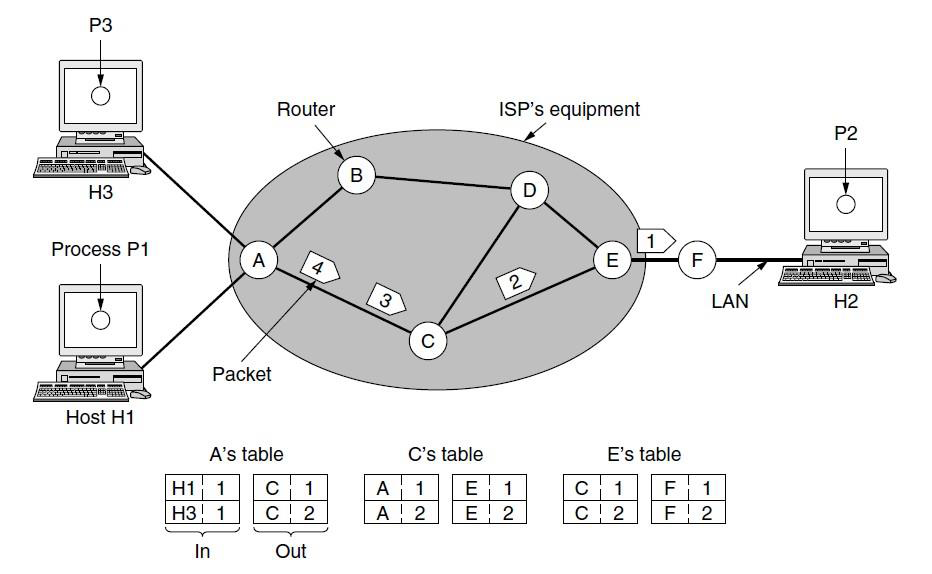
Question No. 2

Comparison of Virtual-Circuit and Data gram Networks

Answer:

Both virtual circuits and data grams have their supporters and their detractors. We will now attempt to summarize both sets of arguments. The major issues are listed in Fig, although purists could probably find a counterexample for everything in the figure.

Datagram Approach: Connectionless Service

When the Internet started, to make it simple, the network layer was designed to provide a connectionless service in which the network-layer protocol treats each packet independently, with each packet having no relationship to any other packet. The idea was that the network layer is only responsible for delivery of packets from the source to the destination. Id this approach, the packets in a message mayor may not travel the same path to their destination. Figure shows the idea. When the network layer provides a connectionless service, each packet traveling in the Internet is an independent entity; there is no relationship between packets belonging to the same

message. The switches in this type of network are called routers. A packet belonging to a message may be followed by a packet belonging to the same message or to a different message. A packet may be followed by a packet coming from the same or from a different source.

Each packet is routed based on the information contained in its header: source and destination addresses. The destination address defines where it should go; the source address defines where it comes from. The router in this case routes the packet based only on the destination address. The source address may be used to send an error message to the source if the packet is discarded. Figure 18.4 shows the forwarding process in a router in this case. We have used symbolic addresses such as A and B.

Virtual-Circuit Approach: Connection-Oriented Service

In a connection-oriented service (also called virtual-circuit approach), there is a relationship between all packets belonging to a message. Before all datagrams in a message can be sent, a virtual connection should be set up to define the path for the datagrams. After connection setup, the datagrams can all follow the same path. In this type of service, not only must the packet contain the source and destination addresses, it must also contain a flow label, a virtual circuit identifier that defines the virtual path the packet should follow. Shortly, we will show how this flow label is determined, but for the moment, we assume that the packet carries this label. Although it looks as though the use of the label may make the source and destination addresses unnecessary during the data transfer phase, parts of the Internet at the network layer still keep these addresses. One reason is that part of the packet path may still be using the connectionless service. Another reason is that the protocol at the network layer is designed with these addresses, and it may take a while before they can be changed. Figure shows the concept of connection- oriented service.

Each packet is forwarded based on the label in the packet. To follow the idea of connection- oriented design to be used in the Internet, we assume that the packet has a label when it reaches the router. Figure 18.6 shows the idea. In this case, the forwarding decision is based on the value of the label, or virtual circuit identifier, as it is sometimes called. To create a connection-oriented service, a three-phase process is used: setup, data transfer, and teardown. In the setup phase, the source and destination addresses of the sender and receiver are used to make table entries for the connection-oriented service. In the teardown phase, the source and destination inform the router to delete the corresponding entries. Data transfer occurs between these two phases.

Question No. 3

Explain about the ROUTING ALGORITHMS .

Answer:

     The main function of the network layer is routing packets from the source machine to the destination machine. In most networks, packets will require multiple hops to make the journey. The only notable exception is for broadcast networks, but even here routing is an issue if the source and destination are not on the same network segment. The algorithms that choose the routes and the data structures that they use are a major area of network layer design.

      The routing algorithm is that part of the network layer software responsible for deciding which output line an incoming packet should be transmitted on. If the network uses datagrams internally, this decision must be made anew for every arriving data packet since the best route may have changed since last time. If the network uses virtual circuits internally, routing decisions are made only when a new virtual circuit is being set up. Thereafter, data packets just follow the already established route. The latter case is sometimes called session routing because

     a route remains in force for an entire session (e.g., while logged in over a VPN). It is sometimes useful to make a distinction between routing, which is making the decision which routes to use, and forwarding, which is what happens when a packet arrives. One can think of a router as having two processes inside it. One of them handles each packet as it arrives, looking up the outgoing line to use for it in the routing tables. This process is forwarding. The other process is responsible for filling in and updating the routing tables. That is where the routing algorithm comes into play.

       Regardless of whether routes are chosen independently for each packet sent or only when new connections are established, certain properties are desirable in a routing algorithm: correctness, simplicity, robustness, stability, fairness, and efficiency. Correctness and simplicity hardly require comment, but the need for robustness may be less obvious at first. Once a major network comes on the air, it may be expected to run continuously for years without system-wide failures. During that period there will be hardware and software failures of all kinds. Hosts, routers, and lines will fail repeatedly, and the topology will change many times. The routing algorithm should be able to cope with changes in the topology and traffic without requiring all jobs in all hosts to be aborted. Imagine the havoc if the network needed to be rebooted every time some router crashed! Stability is also an important goal for the routing algorithm. There exist routing algorithms that never converge to a fixed set of paths, no matter how long they run. A stable algorithm reaches equilibrium and stays there. It should converge quickly too, since communication may be disrupted until the routing algorithm has reached equilibrium. Fairness and efficiency may sound obvious—surely no reasonable person would oppose them—but as it turns out, they are often contradictory goals. As a simple example of this conflict, look at Fig. Suppose that there is enough traffic between A and A′, between B and B′, and between C and C′ to saturate the horizontal links. To maximize the total flow, the X to X′ traffic should be shut off altogether. Unfortunately, X and X′ may not see it that way. Evidently, some compromise between global efficiency and fairness to individual connections is needed. Before we can even attempt to find trade-offs between fairness and efficiency, we must decide what it is we seek to optimize. Minimizing the mean packet delay is an obvious candidate to send traffic through the network effectively, but so is maximizing total network throughput. Furthermore, these two goals are also in conflict, since operating any queuing system near capacity implies a long queuing delay. As a compromise, many networks attempt to minimize the distance a packet must travel, or simply reduce the number of hops a packet must make. Either choice tends to improve the delay and also reduce the amount of bandwidth consumed per packet, which tends to improve the overall network throughput as well.

   Routing algorithms can be grouped into two major classes: non adaptive and adaptive. Non adaptive algorithms do not base their routing decisions on any measurements or estimates of the current topology and traffic. Instead, the choice of the route to use to get from I to J (for all I and J) is computed in advance, offline, and downloaded to the routers when the network is booted. This procedure is sometimes called static routing. Because it does not respond to failures, static routing is mostly useful for situations in which the routing choice is clear. For example, router F in Fig. should send packets headed into the network to router E regardless of the ultimate destination. Adaptive algorithms, in contrast, change their routing decisions to reflect changes in the topology, and sometimes changes in the traffic as well.

These dynamic routing algorithms differ in where they get their information (e.g., locally, from adjacent routers, or from all routers), when they change the routes(e.g., when the topology T seconds as the load changes), and what metric is used for optimization

(e.g., distance, number of hops, or estimated transit time).In the following sections, we will discuss a variety of routing algorithms. The algorithms cover delivery models besides sending a packet from a source to a destination. Sometimes the goal is to send the packet to multiple, all, or one of a set of destinations. All of the routing algorithms we describe here make decisions based on the topology; we defer the possibility of decisions based on the traffic levels to Sec.

The Optimality Principle

Before we get into specific algorithms, it may be helpful to note that one can make a general statement about optimal routes without regard to network topology or traffic. This statement is known as the optimality principle (Bellman, 1957). It states that if router J is on the optimal path from router I to router K, then the optimal path from J to K also falls along the same route. To see this, call the part of the route from I to J r1 and the rest of the route r 2. If a route better than r 2 existed from J to K, it could be concatenated with r 1 to improve the route from I to K, contradicting our statement that r 1r 2 is optimal. As a direct consequence of the optimality principle, we can see that the set of optimal routes from all sources to a given destination form a tree rooted at the destination. Such a tree is called a sink tree and is illustrated in Fig. where the distance metric is the number of hops. The goal of all routing algorithms is to discover and use the sink trees for all routers.

(a) A network. (b) A sink tree for router B.

Note that a sink tree is not necessarily unique; other trees with the same path lengths may exist. If we allow all of the possible paths to be chosen, the tree becomes a more general structure called a DAG (Directed Acyclic Graph). DAGs have no loops. We will use sink trees as convenient shorthand for both cases. Both cases also depend on the technical assumption that the paths do not interfere with each other so, for example, a traffic jam on one path will not cause another path to divert. Since a sink tree is indeed a tree, it does not contain any loops, so each

packet will be delivered within a finite and bounded number of hops. In practice, life is not quite this easy. Links and routers can go down and come back up during operation, so different routers may have different ideas about the current topology. Also, we have quietly finessed the issue of whether each router has to individually acquire the information on which to base its sink tree computation or whether this information is collected by some other means. We will come back to these issues shortly. Nevertheless, the optimality principle and the sink tree provide a benchmark against which other routing algorithms can be measured.

Question No. 4

Explain about the Shortest Path Algorithm.

Answer:

Let us begin our study of routing algorithms with a simple technique for computing optimal paths given a complete picture of the network. These paths are the ones that we want a distributed routing algorithm to find, even though not all routers may know all of the details of the network. The idea is to build a graph of the network, with each node of the graph representing a router and each edge of the graph representing a communication line, or link. To choose a route between a given pair of routers, the algorithm just finds the shortest path between them on the graph.

The concept of a shortest path deserves some explanation. One way of measuring path length is the number of hops. Using this metric, the paths ABC and ABE in Fig. are equally long. Another metric is the geographic distance in kilometers, in which case ABC is clearly much longer than ABE (assuming the figure is drawn to scale).

The first six steps used in computing the shortest path from A to D. The arrows indicate the working node.

However, many other metrics besides hops and physical distance are also possible. For example, each edge could be labeled with the mean delay of a standard test packet, as measured by hourly runs. With this graph labeling, the shortest path is the fastest path rather than the path with the fewest edges or kilometers. In the general case, the labels on the edges could be computed as a function of the distance, bandwidth, average traffic, communication cost, measured delay, and other factors. By changing the weighting function, the algorithm would then compute the

‘‘shortest’’ path measured according to any one of a number of criteria or to a combination of criteria. Several algorithms for computing the shortest path between two nodes of a graph are known. This one is due to Dijkstra (1959) and finds the shortest paths between a source and all destinations in the network. Each node is labeled (in parentheses) with its distance from the source node along the best known path. The distances must be non-negative, as they will be if they are based on real quantities like bandwidth and delay. Initially, no paths are known, so all nodes are labeled with infinity. As the algorithm proceeds and paths are found, the labels may change, reflecting better paths. A label may be either tentative or permanent. Initially, all labels are tentative. When it is discovered that a label represents the shortest possible path from the source to that node, it is made permanent and never changed thereafter. To illustrate how the labeling algorithm works, look at the weighted, undirected graph of Fig., where the weights represent, for example, distance. We want to find the shortest path from A to D. We start out by marking node A as permanent, indicated by a filled-in circle. Then we examine, in turn, each of the nodes adjacent to A (the working node), relabeling each one with the distance to A. Whenever a node is relabeled, we also label it with the node from which the probe was made so that we can reconstruct the final path later. If the network had more than one shortest path from A to D and we wanted to find all of them, we would need to remember all of the probe nodes that could reach a node with the same distance. Having examined each of the nodes adjacent to A, we examine all the tentatively labeled nodes in the whole graph and make the one with the smallest label permanent, as shown in Fig. (b). this one becomes the new working node. We now start at B and examine all nodes adjacent to it. If the sum of the label on B and the distance from B to the node being considered is less than the label on that node, we have a shorter path, so the node is relabeled. After all the nodes adjacent to the working node have been inspected and the tentative labels changed if possible, the entire graph is searched for the tentatively labeled node with the smallest value. This node is made permanent and becomes the working node for the next round. Figure shows the first six steps of the algorithm. To see why the algorithm works, look at Fig. (c). At this point we have just made E permanent. Suppose that there were a shorter path than ABE, say AXYZE (for some X and Y). There are two possibilities: either node Z has already been made permanent, or it has not been. If it has, then E has already been probed (on the round following the one when Z was made permanent), so the AXYZE path has not escaped our attention and thus cannot be a shorter path. Now consider the case where Z is still tentatively labeled. If the label at Z is greater than or equal to that at E, then AXYZE cannot be a shorter path than ABE. If the label is less than that of E, then Z and not E will become permanent first, allowing E to be probed from Z. This algorithm is given in Fig. The global variables n and dist describe the graph and are initialized before shortest path is called. The only difference between the program and the algorithm described above is that in Fig., we compute the shortest path starting at the terminal node, t, rather than at the source node, s. Since the shortest paths from t to s in an undirected graph are the same as the shortest paths from s to t, it does not matter at which end we begin. The reason for searching backward is that each node is labeled with its predecessor rather than its successor. When the final path is copied into the output variable, path, the path is thus reversed. The two reversal effects cancel, and the answer is produced in the correct order.

Question No. 5

 Explain the followings in detail.

a)Flooding

b)Distance Vector Routing

c)The Count-to-Infinity Problem

d)Hierarchical Routing

e)CONGESTION CONTROL ALGORITHMS

f)Admission Control

Answer:

Flooding

When a routing algorithm is implemented, each router must make decisions based on local knowledge, not the complete picture of the network. A simple local technique is flooding, in

which every incoming packet is sent out on every outgoing line except the one it arrived on. Flooding obviously generates vast numbers of duplicate packets, in fact, an infinite number unless some measures are taken to damp the process. One such measure is to have a hop counter contained in the header of each packet that is decremented at each hop, with the packet being discarded when the counter reaches zero. Ideally, the hop counter should be initialized to the length of the path from source to destination. If the sender does not know how long the path is, it can initialize the counter to the worst case, namely, the full diameter of the network.

Flooding with a hop count can produce an exponential number of duplicate packets as the hop count grows and routers duplicate packets they have seen before. A better technique for damming the flood is to have routers keep track of which packets have been flooded, to avoid sending them out a second time. One way to achieve this goal is to have the source router put a sequence number in each packet it receives from its hosts. Each router then needs a list per source router telling which sequence numbers originating at that source have already been seen. If an incoming packet is on the list, it is not flooded.

#define MAX NODES 1024 /* maximum number of nodes */

#define INFINITY 1000000000 /* a number larger than every maximum path */ int n, dist[MAX NODES][MAX NODES]; /* dist[i][j] is the distance from i to j */ void shortest path(int s, int t, int path[])

{ struct state { /* the path being worked on */ int predecessor; /* previous node */

int length; /* length from source to this node */ enum {permanent, tentative} label; /* label state */

} state[MAX NODES];

int i, k, min; struct state *p;

for (p = &state[0]; p < &state[n]; p++) { /* initialize state */ p->predecessor = −1;

p->length = INFINITY; p->label = tentative;

}

state[t].length = 0; state[t].label = permanent; k = t; /* k is the initial working node */

do { /* Is there a better path from k? */

for (i = 0; i < n; i++) /* this graph has n nodes */ if (dist[k][i] != 0 && state[i].label == tentative) { if (state[k].length + dist[k][i] < state[i].length) { state[i].predecessor = k;

state[i].length = state[k].length + dist[k][i];

}

}

/* Find the tentatively labeled node with the smallest label. */ k = 0; min = INFINITY;

for (i = 0; i < n; i++)

if (state[i].label == tentative && state[i].length < min) { min = state[i].length;

k = i;

}

state[k].label = permanent;

} while (k != s);

/* Copy the path into the output array. */ i = 0; k = s;

do {path[i++] = k; k = state[k].predecessor; } while (k >= 0);

}

Dijkstra’s algorithm to compute the shortest path through a graph

      To prevent the list from growing without bound, each list should be augmented by a counter, k, meaning that all sequence numbers through k have been seen. When a packet comes in, it is easy to check if the packet has already been flooded (by comparing its sequence number to k; if so, it is discarded. Furthermore, the full list below k is not needed, since k effectively summarizes it. Flooding is not practical for sending most packets, but it does have some important uses. First, it ensures that a packet is delivered to every node in the network. This may be wasteful if there is a single destination that needs the packet, but it is effective for broadcasting information. In wireless networks, all messages transmitted by a station can be received by all other stations within its radio range, which is, in fact, flooding, and some algorithms utilize this property. Second, flooding is tremendously robust. Even if large numbers of routers are blown to bits (e.g., in a military network located in a war zone), flooding will find a path if one exists, to get a packet to its destination. Flooding also requires little in the way of setup. The routers only need to know their neighbors. This means that flooding can be used as a building block for other routing algorithms that are

more efficient but need more in the way of setup. Flooding can also be used as a metric against which other routing algorithms can be compared. Flooding always chooses the shortest path because it chooses every possible path in parallel. Consequently, no other algorithm can produce a shorter delay (if we ignore the overhead generated by the flooding process itself).

b)Distance Vector Routing

Computer networks generally use dynamic routing algorithms that are more complex than flooding, but more efficient because they find shortest paths for the current topology. Two dynamic algorithms in particular, distance vector routing and link state routing, are the most popular. In this section, we will look at the former algorithm. In the following section, we will study the latter algorithm. A distance vector routing algorithm operates by having each router maintain a table (i.e., a vector) giving the best known distance to each destination and which link to use to get there. These tables are updated by exchanging information with the neighbors. Eventually, every router knows the best link to reach each destination. The distance vector routing algorithm is sometimes called by other names, most commonly the distributed Bellman- Ford routing algorithm, after the researchers who developed it (Bellman, 1957; and Ford and Fulkerson, 1962). It was the original ARPANET routing algorithm and was also used in the Internet under the name RIP. In distance vector routing, each router maintains a routing table indexed by, and containing one entry for each router in the network. This entry has two parts: the preferred outgoing line to use for that destination and an estimate of the distance to that destination. The distance might be measured as the number of hops or using another metric, as we discussed for computing shortest paths. The router is assumed to know the ‘‘distance’’ to meach of its neighbors. If the metric is hops, the distance is just one hop. If the metric is propagation delay, the router can measure it directly with special ECHO packets that the receiver just timestamps and sends back as fast as it can. As an example, assume that delay is used as a metric and that the router knows the delay to each of its neighbors. Once every T m sec, each router sends to each neighbor a list of its estimated delays to each destination. It also receives a similar list from each neighbor. Imagine that one of these tables has just come in from neighbor X, with Xi being X’s estimate of how long it takes to get to router i.If the router knows that the  delay to X is m m sec, it also knows that it can reach router i via X in Xi msec. By performing this calculation for each neighbor, a router can find out which estimate seems the best and use that estimate and the corresponding link in its new routing table. Note that the old routing table is not used in the calculation. This updating process is illustrated in Fig. 5-9. Part (a) shows a network. The first four columns of part (b) show the delay vectors received from the neighbors of router J. A claims to have a 12-msec delay to B, a 25-msec delay to C, a 40-msec delay to D, etc. Suppose that J has measured or estimated its delay to its neighbors, A, I, H, and K, as 8, 10, 12, and 6 m sec, respectively.

(a) A network. (b) Input from A, I, H, K, and the new routing table for J.

c)The Count-to-Infinity Problem

The settling of routes to best paths across the network is called convergence. Distance vector routing is useful as a simple technique by which routers can collectively compute shortest paths, but it has a serious drawback in practice: although it converges to the correct answer, it may do so slowly. In particular, it reacts rapidly to good news, but leisurely to bad news. Consider a router whose best route to destination X is long. If, on the next exchange, neighbor A suddenly reports a short delay to X, the router just switches over to using the line to A to send traffic to X. In one vector exchange, the good news is processed. To see how fast good news propagates, consider the five-node (linear) network of Fig. 5-10, where the delay metric is the number of hops. Suppose A is down initially and all the other routers know this. In other words, they have all recorded the delay to A as infinity.

When A comes up, the other routers learn about it via the vector exchanges. For simplicity, we will assume that there is a gigantic going somewhere that is struck periodically to initiate a vector exchange at all routers simultaneously. At the time of the first exchange, B learns that its left-hand neighbor has zero delay to A. B now makes an entry in its routing table indicating that A is one hop away to the left. All the other routers still think that A is down. At this point, the routing table entries for A are as shown in the second row of Fig. (a). On the next exchange, C learns that B has a path of length 1 to A, so it updates its routing table to indicate a path of length 2, but D and E do not hear the good news until later. Clearly, the good news is spreading at the rate of one hop per exchange. In a network whose longest path is of length N hops, within N exchanges everyone will know about newly revived links and routers. Now let us consider the situation of (b), in which all the links and routers are initially up. Routers B, C, D, and E have distances to A of 1, 2, 3, and 4 hops, respectively. Suddenly, either A goes down or the link between A and B is cut (which is effectively the same thing from B’s point of view).At the first packet exchange, B does not hear anything from A. Fortunately, C says ‘‘Do not worry; I have a path to A of length 2.’’ Little does B suspect that C’s path runs through B itself . For all B knows, C might have ten links all with separate paths to A of length 2. As a result, B thinks it can reach A via C, with a path length of 3. D and E do not update their entries for A on the first exchange.

On the second exchange, C notices that each of its neighbors claims to have a path to A of length

3. It picks one of them at random and makes its new distance to A 4, as shown in the third row of Fig. 5-10(b). Subsequent exchanges produce the history shown in the rest of Fig. 5-10(b).From this figure, it should be clear why bad news travels Slowly: no router ever has a value more than one higher than the minimum of all its neighbors. Gradually, all routers work their way up to infinity, but the number of exchanges required depends on the numerical value used for infinity. For this reason, it is wise to set infinity to the longest path plus 1.Not entirely surprisingly, this problem is known as the count-to-infinity problem. There have been many attempts to solve it, for example, preventing routers from advertising their best paths back to the neighbors from which they heard them with the split horizon with poisoned reverse rule discussed in RFC 1058.However, none of these heuristics work well in practice despite the colorful names. The core of the problem is that when X tells Y that it has a path somewhere, Y has no way of knowing whether it itself is on the path.
d)Hierarchical Routing
As networks grow in size, the router routing tables grow proportionally. Not only is router memory consumed by ever-increasing tables, but more CPU time is needed to scan them and more bandwidth is needed to send status reports about them. At a certain point, the network may grow to the point where it is no longer feasible for every router to have an entry for every other router, so the routing will have to be done hierarchically, as it is in the telephone network. When hierarchical routing is used, the routers are divided into what we will call regions. Each router knows all the details about how to route packets to destinations within its own region but knows nothing about the internal structure of other regions. When different networks are interconnected, it is natural to regard each one as a separate region to free the routers in one network from having to know the topological structure of the other ones. For huge networks, a two-level hierarchy may be insufficient; it may be necessary to group the regions into clusters, the clusters into zones, the zones into groups, and so on, until we run out of names for aggregations. As an example of a multilevel hierarchy, consider how a packet might be routed from Berkeley, California, to Malindi, Kenya. The Berkeley router would know the detailed topology within California but would send all out-of-state traffic to the Los Angeles router. The Los Angeles router would be able to route traffic directly to other domestic routers but would send all foreign traffic to New York. The New York router would be programmed to direct all traffic to the router in the destination country responsible for handling foreign traffic, say, in Nairobi. Finally, the packet would work its way down the tree in Kenya until it got to Malindi. Figure gives a quantitative example of routing in a two-level hierarchy with five regions. The full routing table for router 1A has 17 entries, as shown in Fig. (b). When routing is done hierarchically, as in Fig. 5-14(c), there are entries for all the local routers, as before, but all other regions are condensed into a single router, so all traffic for region 2 goes via the 1B-2A line, but the rest of the remote traffic goes via the 1C-3B line. Hierarchical routing has reduced the table from 17 to 7 entries. As the ratio of the number of regions to the number of routers per region grows, the savings in table space increase. Unfortunately, these gains in space are not free. There is a penalty to be paid: increased path length. For example, the best route from 1A to 5C is via region 2,but with hierarchical routing all traffic to region 5 goes via region 3, because that is better for most destinations in region 5.When a single network becomes very large, an interesting question is ‘‘how many levels should the hierarchy have?’’ For example, consider a network with 720 routers. If there is no hierarchy, each router needs 720 routing table entries. If the network is partitioned into 24 regions of 30 routers each, each router needs 30 local entries plus 23 remote entries for a total of 53 entries. If a three-level hierarchy is chosen, with 8 clusters each containing 9 regions of 10 routers, each router needs 10 entries for local routers, 8 entries for routing to other regions within its own cluster, and 7 entries for distant clusters, for a total of 25 entries.Kamoun and Kleinrock (1979) discovered that the optimal number of levels for an N router network is ln N, requiring a total of e ln N entries per router. They have also shown that the increase in effective mean path length caused by hierarchical routing is sufficiently small that it is usually acceptable.

e)CONGESTION CONTROL ALGORITHMS

Too many packets present in (a part of) the network causes packet delay and loss that degrades performance. This situation is called congestion. The network and transport layers share the responsibility for handling congestion. Since congestion occurs within the network, it is the network layer that directly experiences it and must ultimately determine what to do with the excess packets. However, the most effective way to control congestion is to reduce the load that the transport layer is placing on the network. This requires the network and transport layers to work together. In this chapter we will look at the network aspects of congestion. In Chap. 6, we will complete the topic by covering the transport aspects of congestion. Figure depicts the onset of congestion. When the number of packets hosts send into the network is well within its carrying capacity, the number delivered is proportional to the number sent. If twice as many are sent, twice as many are delivered. However, as the offered load approaches the carrying capacity, bursts of traffic occasionally fill up the buffers inside routers and some packets are lost. These lost packets consume some of the capacity, so the number of delivered packets falls below the ideal curve. The network is now congested.

With too much traffic, performance drops sharply.

Unless the network is well designed, it may experience a congestion collapse, in which performance plummets as the offered load increases beyond the capacity. This can happen

because packets can be sufficiently delayed inside the network that they are no longer useful when they leave the network. For example, in the early Internet, the time a packet spent waiting for a backlog of packets ahead of it to be sent over a slow 56-kbps link could reach the maximum time it was allowed to remain in the network. It then had to be thrown away. A different failure mode occurs when senders retransmit packets that are greatly delayed, thinking that they have been lost. In this case, copies of the same packet will be delivered by the network, again wasting its capacity. To capture these factors, the y-axis of Fig. is given as good put, which is the rate at which useful packets are delivered by the network. We would like to design networks that avoid congestion where possible and do not suffer from congestion collapse if they do become congested. Unfortunately, congestion cannot wholly be avoided. If all of a sudden, streams of packets begin arriving on three or four input lines and all need the same output line, a queue will build up. If there is insufficient memory to hold all of them, packets will be lost. Adding more memory may help up to a point, but Nagle (1987) realized that if routers have an infinite amount of memory, congestion gets worse, not better. This is because by the time packets get to the front of the queue, they have already timed out (repeatedly) and duplicates have been sent. This makes matters worse, not better—it leads to congestion collapse. Low-bandwidth links or routers that process packets more slowly than the line rate can also become congested. In this case, the situation can be improved by directing some of the traffic away from the bottleneck to other parts of the network. Eventually, however, all regions of the network will be congested. In this situation, there is no alternative but to shed load or build a faster network. It is worth pointing out the difference between congestion control and flow control, as the relationship is a very subtle one. Congestion control has to do with making sure the network is able to carry the offered traffic. It is a global issue, involving the behavior of all the hosts and routers. Flow control, in contrast, relates to the traffic between a particular sender and a particular receiver. Its job is to make sure that a fast sender cannot continually transmit data faster than the receiver is able to absorb it. To see the difference between these two concepts, consider a network made up of 100- Gbps fiber optic links on which a supercomputer is trying to force feed a large file to a personal computer that is capable of handling only 1 Gbps. Although there is no congestion (the network itself is not in trouble), flow control is needed to force the supercomputer to stop frequently to give the personal computer chance to breathe. At the other extreme, consider a network with 1- Mbps lines and 1000 large computers, half of which are trying to transfer files at 100 kbps to the other half. Here, the problem is not that of fast senders overpowering slow receivers, but that the total offered traffic exceeds what the network can handle.

The reason congestion control and flow control are often confused is that the best way to handle both problems is to get the host to slow down. Thus, a host can get a ‘‘slow down’’ message either because the receiver cannot handle the load or because the network cannot handle it. We will come back to this point in Chap. 6. We will start our study of congestion control by looking at the approaches that can be used at different time scales. Then we will look at approaches to preventing congestion from occurring in the first place, followed by approaches for coping with it once it has set in.

f)Admission Control

One technique that is widely used in virtual-circuit networks to keep congestion at bay is admission control. The idea is simple: do not set up a new virtual circuit unless the network can carry the added traffic without becoming congested. Thus, attempts to set up a virtual circuit may fail. This is better than the alternative, as letting more people in when the network is busy just makes matters worse. By analogy, in the telephone system, when a switch gets overloaded it practices admission control by not giving dial tones. The trick with this approach is working out when a new virtual circuit will lead to congestion. The task is straightforward in the telephone network because of the fixed bandwidth of calls (64 kbps for uncompressed audio). However, virtual circuits in computer networks come in all shapes and sizes. Thus, the circuit must come with some characterization of its traffic if we are to apply admission control. Traffic is often described in terms of its rate and shape. The problem of how to describe it in a simple yet 

meaningful way is difficult because traffic is typically bursty—the average rate is only half the story. For example, traffic that varies while browsing the Web is more difficult to handle than a streaming movie with the same long-term throughput because the bursts of Web traffic are more likely to congest routers in the network. A commonly used descriptor that captures this effect is the leaky bucket or token bucket. A leaky bucket has two parameters that bound the average rate and the instantaneous burst size of traffic. Since leaky buckets are widely used for quality of service, we will go over them in detail in Sec. Armed with traffic descriptions, the network can decide whether to admit the new virtual circuit. One possibility is for the network to reserve enough capacity along the paths of each of its virtual circuits that congestion will not occur. In this case, the traffic description is a service agreement for what the network will guarantee its users. We have prevented congestion but veered into the related topic of quality of service a little too early; we will return to it in the next section. Even without making guarantees, the network can use traffic descriptions for admission control. The task is then to estimate how many circuits will fit within the carrying capacity of the network without congestion. Suppose that virtual circuits that may blast traffic at rates up to 10 Mbps all pass through the same 100-Mbps physical link. How many circuits should be admitted? Clearly, 10 circuits can be admitted without risking congestion, but this is wasteful in the normal case since it may rarely happen that all 10 are transmitting full blast at the same time. In real networks, measurements of past behavior that capture the statistics of transmissions can be used to estimate the number of circuits to admit, to trade better performance for acceptable risk. Admission control can also be combined with traffic-aware routing by considering routes around traffic hotspots as part of the setup procedure. For example, consider the network illustrated in Fig (a), in which two routers are congested, as indicated.

(a) A congested network. (b) The portion of the network that is not congested. A virtual circuit from A to B is also shown.

Suppose that a host attached to router A wants to set up a connection to a host attached to router

B. Normally, this connection would pass through one of the congested routers. To avoid this situation, we can redraw the network as shown in Fig. 5-24(b), omitting the congested routers and all of their lines. The dashed line shows a possible route for the virtual circuit that avoids the congested routers. Shaikh et al. (1999) give a design for this kind of load-sensitive routing.

UNIT - IV

Inter-networking

Until now, we have implicitly assumed that there is a single homogeneous network, with each machine using the same protocol in each layer. Unfortunately, this assumption is wildly optimistic. Many different networks exist, including PANs, LANs, MANs, and WANs. We have described Ethernet, Internet over cable, the fixed and mobile telephone networks, 802.11, 802.16, and more. Numerous protocols are in widespread use across these networks in every layer. In the following sections, we will take a careful look at the issues that arise when two or more networks are connected to form an inter network, or more simply an internet.

It would be much simpler to join networks together if everyone used a single networking technology, and it is often the case that there is a dominant kind of network, such as Ethernet. Some pundits speculate that the multiplicity of technologies will go away as soon as everyone realizes how wonderful [fill in your favorite network] is. Do not count on it. History shows this to be wishful thinking. Different kinds of networks grapple with different problems, so, for example, Ethernet and satellite networks are always likely to differ. Reusing existing systems, such as running data networks on top of cable, the telephone network, and power lines, adds constraints that cause the features of the networks to diverge. Heterogeneity is here to stay. If there will always be different networks, it would be simpler if we did not need to interconnect them. This also is unlikely. Bob Metcalfe postulated that the value of a network with N nodes is the number of connections that may be made between the nodes, or N2 (Gilder, 1993).

This means that large networks are much more valuable than small networks because they allow many more connections, so there always will be an incentive to combine smaller networks. The Internet is the prime example of this interconnection. (We will write Internet with a capital ‘‘I’’ to distinguish it from other internets, or connected networks.)The purpose of joining all these networks is to allow users on any of them to communicate with users on all the other ones. When you pay an ISP for Internet service, you may be charged depending on the bandwidth of your line, but what you are really paying for is the ability to exchange packets with any other host that is also connected to the Internet. After all, the Internet would not be very popular if you could only send packets to other hosts in the same city. Since networks often differ in important ways, getting packets from one network to another is not always so easy. We must address problems of heterogeneity, and also problems of scale as the resulting internet grows very large. We will begin by looking at how networks can differ to see what we are up against. Then we shall see the approach used so successfully by IP (Internet Protocol), the network layer protocol of the Internet, including techniques for tunneling through networks, routing in internetworks, and packet fragmentation.

Question No. 1

What Tunneling. Explain in detail? 

Answer:

Handling the general case of making two different networks interwork is exceedingly difficult. However, there is a common special case that is manageable even for different network protocols. This case is where the source and destination hosts are on the same type of network, but there is a different network in between. As an example, think of an international bank with an IPv6 network in Paris, an IPv6 network in London and connectivity between the offices via the IPv4 Internet. This situation is shown in Fig.

The solution to this problem is a technique called tunneling. To send an IP packet to a host in the London office, a host in the Paris office constructs the packet containing an IPv6 address in London, and sends it to the multiprotocol router that connects the Paris IPv6 network to the IPv4 Internet. When this router gets the IPv6 packet, it encapsulates the packet with an IPv4 header addressed to the IPv4 side of the multiprotocol router that connects to the London IPv6 network.

That is, the router puts a (IPv6) packet inside a (IPv4) packet. When this wrapped packet arrives, the London router removes the original IPv6 packet and sends it onward to the destination host.

The path through the IPv4 Internet can be seen as a big tunnel extending from one multiprotocol router to the other. The IPv6 packet just travels from one end of the tunnel to the other, snug in its nice box. It does not have to worry about dealing with IPv4 at all. Neither do the hosts in Paris or London. Only the multiprotocol routers have to understand both IPv4 and IPv6 packets. In effect, the entire trip from one multiprotocol router to the other is like a hop over a single link.

An analogy may make tunneling clearer. Consider a person driving her car from Paris to London. Within France, the car moves under its own power, but when it hits the English Channel, it is loaded onto a high-speed train and transported to England through the Chunnel (cars are not permitted to drive through the Chunnel). Effectively, the car is being carried as freight, as depicted in Fig. At the far end, the car is let loose on the English roads and once again continues to move under its own power. Tunneling of packets through a foreign network works the same way. Tunneling is widely used to connect isolated hosts and networks using other networks. The network that results is called an overlay since it has effectively been overlaid on the base network. Deployment of a network protocol with a new feature is a common reason, as our ‘‘IPv6 over IPv4’’ example shows. The disadvantage of tunneling is that none of the hosts on the network that are tunneled over can be reached because the packets cannot escape in the middle of the tunnel.

Question No 2

Explain about Inter-network Routing?

Answer:

Routing through an internet poses the same basic problem as routing within a single network, but with some added complications. To start, the networks may internally use different routing algorithms. For example, one network may use link state routing and another distance vector routing. Since link state algorithms need to know the topology but distance vector algorithms do not, this difference alone would make it unclear how to find the shortest paths across the internet. Networks run by different operators lead to bigger problems. First, the operators may have different ideas about what is a good path through the network. One operator may want the route with the least delay, while another may want the most inexpensive route. This will lead the operators to use different quantities to set the shortest-path costs (e.g., milliseconds of delay vs. monetary cost). The weights will not be comparable across networks, so shortest paths on the internet will not be well defined. Worse yet, one operator may not want another operator to even know the details of the paths in its network, perhaps because the weights and paths may reflect sensitive information (such as the monetary cost) that represents a competitive business advantage. Finally, the internet may be much larger than any of the networks that comprise it. It may therefore require routing algorithms that scale well by using a hierarchy; even if none of the individual networks need to use a hierarchy. All of these considerations lead to a two-level routing algorithm. Within each network, an intra domain or interior gateway protocol is used for routing.(‘‘Gateway’’ is an older term for ‘‘router.’’) It might be a link state protocol of the kind we have already described. Across the networks that make up the internet, an inter domain or exterior gateway protocol is used. The networks may all use different intra domain protocols, but they must use the same inter domain protocol. In the Internet, the inter domain routing protocol is called BGP (Border Gateway Protocol).

       We will there is one more important term to introduce. Since each network is operated independently of all the others, it is often referred to as an AS (Autonomous System). A good mental model for an AS is an ISP network. In fact, an ISP network may be comprised of more than one AS, if it is managed, or, has been acquired, as multiple networks. But the difference is usually not significant. The two levels are usually not strictly hierarchical, as highly suboptimal paths might result if a large international network and a small regional network were both abstracted to be a single network. However, relatively little information about routes within the networks is exposed to find routes across the internetwork.

This helps to address all of the complications. It improves scaling and lets operators freely select routes within their own networks using a protocol of their choosing. It also does not require weights to be compared across networks or expose sensitive information outside of networks. However, we have said little so far about how the routes across the networks of the internet are determined. In the Internet, a large determining factor is the business arrangements between ISPs. Each ISP may charge or receive money from the other ISPs for carrying traffic. Another factor is that if internetwork routing requires crossing international boundaries, various laws may suddenly come into play, such as Sweden’s strict privacy laws about exporting personal data about Swedish citizens from Sweden. All of these nontechnical factors are wrapped up in the concept of a routing policy that governs the way autonomous networks select the routes that they use. We will return to routing policies when we describe BGP.

Question No 3.

what is Packet Fragmentation ?

Answer:

Each network or link imposes some maximum size on its packets. These limits have various causes, among them

1. Hardware (e.g., the size of an Ethernet frame).

2. Operating system (e.g., all buffers are 512 bytes).

3. Protocols (e.g., the number of bits in the packet length field).

4. Compliance with some (inter)national standard.

5. Desire to reduce error-induced retransmissions to some level.

6. Desire to prevent one packet from occupying the channel too long.

The result of all these factors is that the network designers are not free to choose any old maximum packet size they wish. Maximum payloads for some common technologies are 1500 bytes for Ethernet and 2272 bytes for 802.11. IP is more generous, allows for packets as big as 65,515 bytes. Hosts usually prefer to transmit large packets because this reduces packet overheads such as bandwidth wasted on header bytes. An obvious internetworking problem appears when a large packet wants to travel through a network whose maximum packet size is too small. This nuisance has been a persistent issue, and solutions to it have evolved along with much experience gained on the Internet. One solution is to make sure the problem does not occur in the first place. However, this is easier said than done. A source does not usually know the path a packet will take through the network to a destination, so it certainly does not know how small packets must be to get there. This packet size is called the Path MTU (Path Maximum Transmission Unit). Even if the source did know the path MTU, packets are routed independently in a connectionless network such as the Internet. This routing means that paths may suddenly change, which can unexpectedly change the path MTU. The alternative solution to the problem is to allow routers to break up packets into fragments, sending each fragment as a separate network layer packet. However, as every parent of a small child knows, converting a large object into small fragments is considerably easier than the reverse process. (Physicists have even given this effect a name: the second law of thermodynamics.) Packet-switching networks, too, have trouble putting the fragments back together again. Two opposing strategies exist for recombining the fragments back into the original packet. The first strategy is to make fragmentation caused by a ‘‘small packet’’ network transparent to any subsequent networks through which the packet must pass on its way to the ultimate destination. This option is shown in Fig (a). In this approach, when an oversized packet arrives at G1, the router breaks it up into fragments. Each fragment is addressed to the same exit router, G2, where the pieces are recombined. In this way, passage through the small-packet network is made transparent. Subsequent networks are not even aware that fragmentation has occurred.

     Transparent fragmentation is straightforward but has some problems. For one thing, the exit router must know when it has received all the pieces, so either a count field or an ‘‘end of packet’’ bit must be provided. Also, because all packets must exit via the same router so that they can be reassembled, the routes are constrained. By not allowing some fragments to follow one route to the ultimate destination and other fragments a disjoint route, some performance may be lost. More significant is the amount of work that the router may have to do. It may need to

buffer the fragments as they arrive, and decide when to throw them away if not all of the fragments arrive. Some of this work may be wasteful, too, as the packet may pass through a series of small packet networks and need to be repeatedly fragmented and reassembled. The other fragmentation strategy is to refrain from recombining fragments at any intermediate routers. Once a packet has been fragmented, each fragment is

(a) Transparent fragmentation. (b) Nontransparent fragmentation.

treated as though it were an original packet. The routers pass the fragments, as shown in Fig. (b), and reassembly is performed only at the destination host. The main advantage of nontransparent fragmentation is that it requires routers to do less work. IP works this way. A complete design requires that the fragments be numbered in such a way that the original data stream can be reconstructed.

The design used by IP is to give every fragment a packet number (carried on all packets), an absolute byte offset within the packet, and a flag indicating whether it is the end of the packet. An example is shown in Fig. While simple, this design has some attractive properties. Fragments can be placed in a buffer at the destination in the right place for reassembly, even if they arrive out of order.

Fragments can also be fragmented if they pass over a network with a yet smaller MTU. This is shown in Fig. (c). Retransmissions of the packet (if all fragments were not received) can be fragmented into different pieces. Finally, fragments can be of arbitrary size, down to a single byte plus the packet header. In all cases, the destination simply uses the packet number and fragment offset to place the data in the right position, and the end-of-packet flag to determine when it has the complete packet. Unfortunately, this design still has problems. The overhead can be higher than with transparent fragmentation because fragment headers are now carried over some links where they may not be needed. But the real problem is the existence of fragments in the first place. Kent and Mogul (1987) argued that fragmentation is detrimental to performance because, as well as the header overheads, a whole packet is lost if any of its fragments are lost and because fragmentation is more of a burden for hosts than was originally realized.

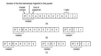
Fragmentation when the elementary data size is 1 byte.

(a) Original packet, containing 10 data bytes.

(b) Fragments after passing through a network with maximum packet size of 8 payload bytes plus header.

(c) Fragments after passing through a size 5 gateway.

This leads us back to the original solution of getting rid of fragmentation in the network, the strategy used in the modern Internet. The process is called path MTU discovery (Mogul and Deering, 1990). It works as follows. Each IP packet is sent with its header bits set to indicate that no fragmentation is allowed to be performed. If a router receives a packet that is too large, it generates an error packet, returns it to the source, and drops the packet. This is shown in Fig. When the source receives the error packet, it uses the information inside to refragment the packet into pieces that are small enough for the router to handle. If a router further down the path has an even smaller MTU, the process is repeated.

The advantage of path MTU discovery is that the source now knows what length packet to send. If the routes and path MTU change, new error packets will be triggered and the source will adapt to the new path. However, fragmentation is still needed between the source and the destination unless the higher layers learn the path MTU and pass the right amount of data to IP. TCP and IP are typically implemented together (as ‘‘TCP/IP’’) to be able to pass this sort of information. Even if this is not done for other protocols, fragmentation has still been moved out of the network and into the hosts. The disadvantage of path MTU discovery is that there may be added startup delays simply to send a packet. More than one round-trip delay may be needed to probe the path and find the MTU before any data is delivered to the destination. This begs the question of whether there are better designs. The answer is probably ‘‘Yes.’’ Consider the design in which each router simply truncates packets that exceed its MTU. This would ensure that the destination learns the MTU as rapidly as possible (from the amount of data that was delivered) and receives some of the data.

Question No 4

Explain about The IP Version 4 Protocol.

Answer:

An appropriate place to start our study of the network layer in the Internet is with the format of the IP datagrams themselves. An IPv4 datagram consists of a header part and a body or payload part. The header has a 20-byte fixed part and a variable-length optional part. The header format is shown in Fig. 5-46. The bits are transmitted from left to right and top to bottom, with the high- order bit of the Version field going first. (This is a ‘‘big-endian’’ network byte order. On little endian machines, such as Intel x86 computers, a software conversion is required on both transmission and reception.) In retrospect, little endian would have been a better choice, but at the time IP was designed, no one knew it would come to dominate computing.

The IPv4 (Internet Protocol) header.

The Version field keeps track of which version of the protocol the datagram belongs to. Version 4 dominates the Internet today, and that is where we have started our discussion. By including the version at the start of each datagram, it becomes possible to have a transition between versions over a long period of time. In fact, IPv6, the next version of IP, was defined more than a decade ago, yet is only just beginning to be deployed. We will describe it later in this section. Its use will eventually be forced when each of China’s almost 231 people has a desktop PC, a laptop, and an IP phone. As an aside on numbering, IPv5 was an experimental real-time stream protocol that was never widely used.

Since the header length is not constant, a field in the header, IHL, is provided to tell how long the header is, in 32-bit words. The minimum value is 5, which applies when no options are present. The maximum value of this 4-bit field is 15, which limits the header to 60 bytes, and thus the Options field to 40 bytes. For some options, such as one that records the route a packet has taken, 40 bytes is far too small, making those options useless. The Differentiated services field is one of the few fields that has changed its meaning (slightly) over the years. Originally, it was called the Type of service field. It was and still is intended to distinguish between different classes of service.

Various combinations of reliability and speed are possible. For digitized voice, fast delivery beats accurate delivery. For file transfer, error-free transmission is more important than fast transmission. The Type of service field provided 3 bits to signal priority and 3 bits to signal whether a host cared more about delay, throughput, or reliability. However, no one really knew what to do with these bits at routers, so they were left unused for many years. When differentiated services were designed, IETF threw in the towel and reused this field. Now, the top 6 bits are used to mark the packet with its service class; we described the expedited and assured

services earlier in this chapter. The bottom 2 bits are used to carry explicit congestion notification information, such as whether the packet has experienced congestion; we described explicit congestion notification as part of congestion control earlier in this chapter. The Total length includes everything in the datagram—both header and data. The maximum length is 65,535 bytes. At present, this upper limit is tolerable, but with future networks, larger datagrams may be needed. The Identification field is needed to allow the destination host to determine which packet a newly arrived fragment belongs to. All the fragments of a packet contain the same Identification value.

Next comes an unused bit, which is surprising, as available real estate in the IP header is extremely scarce. As an April fool’s joke, Bellovin (2003) proposed using this bit to detect malicious traffic. This would greatly simplify security, as packets with the ‘‘evil’’ bit set would be known to have been sent by attackers and could just be discarded. Unfortunately, network security is not this simple. Then come two 1-bit fields related to fragmentation. DF stands for Don’t Fragment. It is an order to the routers not to fragment the packet. Originally, it was intended to support hosts incapable of putting the pieces back together again. Now it is used as part of the process to discover the path MTU, which is the largest packet that can travel along a path without being fragmented. By marking the datagram with the DF bit, the sender knows it will either arrive in one piece, or an error message will be returned to the sender. MF stands for More Fragments. All fragments except the last one have this bit set. It is needed to know when all fragments of a datagram have arrived. The Fragment offset tells where in the current packet this fragment belongs.

All fragments except the last one in a datagram must be a multiple of 8 bytes, the elementary fragment unit. Since 13 bits are provided, there is a maximum of 8192 fragments per datagram, supporting a maximum packet length up to the limit of the Total length field. Working together, the Identification, MF, and Fragment offset fields are used to implement fragmentation as described in Sec. 5.5.5.The TtL (Time to live) field is a counter used to limit packet lifetimes. It was originally supposed to count time in seconds, allowing a maximum lifetime of 255 sec. It must be decremented on each hop and is supposed to be decremented multiple times when a packet is queued for a long time in a router. In practice, it just counts hops. When it hits zero, the packet is discarded and a warning packet is sent back to the source host. This feature prevents packets from wandering around forever, something that otherwise might happen if the routing tables ever become corrupted.

When the network layer has assembled a complete packet, it needs to know what to do with it. The Protocol field tells it which transport process to give the packet to. TCP is one possibility, but so are UDP and some others. The numbering of protocols is global across the entire Internet. Protocols and other assigned numbers were formerly listed in RFC 1700, but nowadays they are contained in an online database located at www.iana.org. Since the header carries vital information such as addresses, it rates its own checksum for protection, the Header checksum. The algorithm is to add up all the 16-bit half words of the header as they arrive, using one’s complement arithmetic, and then take the one’s complement of the result. For purposes of this algorithm, the Header checksum is assumed to be zero upon arrival. Such a checksum is useful for detecting errors while the packet travels through the network. Note that it must be recomputed at each hop because at least one field always changes (the Time to live field), but

tricks can be used to speed up the computation. The Source address and Destination address indicate the IP address of the source and destination network interfaces. The Options field was designed to provide an escape to allow subsequent versions of the protocol to include information not present in the original design, to permit experimenters to try out new ideas, and to avoid allocating header bits to information that is rarely needed. The options are of variable length. Each begins with a 1-byte code identifying the option. Some options are followed by a 1- byte option length field, and then one or more data bytes. The Options field is padded out to a multiple of 4 bytes. Originally, the five options listed in Fig. were defined.

The Security option tells how secret the information is. In theory, a military router might use this field to specify not to route packets through certain countries the military considers to be ‘‘bad guys.’’ In practice, all routers ignore it, so its only practical function is to help spies find the good stuff more easily. The Strict source routing option gives the complete path from source to destination as a sequence of IP addresses. The datagram is required to follow that exact route. It is most useful for system managers who need to send emergency packets when the routing tables have been corrupted, or for making timing measurements. The Loose source routing option requires the packet to traverse the list of routers specified, in the order specified, but it is allowed to pass through other routers on the way. Normally, this option will provide only a few routers, to force a particular path. For example, to force a packet from London to Sydney to go west instead of east, this option might specify routers in New York, Los Angeles, and Honolulu. This option is most useful when political or economic considerations dictate passing through or avoiding certain countries.

Question No 5

Explain about The IP Version 6 Protocol.

Answer:

IP has been in heavy use for decades. It has worked extremely well, as demonstrated by the exponential growth of the Internet. Unfortunately, IP has become a victim of its own popularity: it is close to running out of addresses. Even with CIDR and NAT using addresses more

sparingly, the last IPv4 addresses are expected to be assigned by ICANN before the end of 2012. This looming disaster was recognized almost two decades ago, and it sparked a great deal of discussion and controversy within the Internet community about what to do about it. In this section, we will describe both the problem and several proposed solutions. The only long-term solution is to move to larger addresses. IPv6 (IP version 6) is a replacement design that does just that. It uses 128-bit addresses; a shortage of these addresses is not likely any time in the foreseeable future. However, IPv6 has proved very difficult to deploy. It is a different network layer protocol that does not really interwork with IPv4, despite many similarities. Also, companies and users are not really sure why they should want IPv6 in any case. The result is that IPv6 is deployed and used on only a tiny fraction of the Internet (estimates are 1%) despite having been an Internet Standard since 1998. The next several years will be an interesting time, as the few remaining IPv4 addresses are allocated. Will people start to auction off their IPv4 addresses on eBay? Will a black market in them spring up? Who knows? In addition to the address problems, other issues loom in the background. In its early years, the Internet was largely used by universities, high-tech industries, and the U.S. Government (especially the Dept. of Defense). With the explosion of interest in the Internet starting in the mid-1990s, it began to be used by a different group of people, often with different requirements. For one thing, numerous people with smart phones use it to keep in contact with their home bases. For another, with the impending convergence of the computer, communication, and entertainment industries, it may not be that long before every telephone and television set in the world is an Internet node, resulting in a billion machines being used for audio and video on demand. Under these circumstances, it became apparent that IP had to evolve and become more flexible. Seeing these problems on the horizon, in 1990 IETF started work on a new version of IP, one that would never run out of addresses, would solve a variety of other problems, and be more flexible and efficient as well. Its major goals were:

1. Support billions of hosts, even with inefficient address allocation.

2. Reduce the size of the routing tables.

3. Simplify the protocol, to allow routers to process packets faster.

4. Provide better security (authentication and privacy).

5. Pay more attention to the type of service, particularly for real-time data.

6. Aid multicasting by allowing scopes to be specified.

7. Make it possible for a host to roam without changing its address.

8. Allow the protocol to evolve in the future.

9. Permit the old and new protocols to coexist for years.

The design of IPv6 presented a major opportunity to improve all of the features in IPv4 that fall short of what is now wanted. To develop a protocol that met all these requirements, IETF issued a call for proposals and discussion in RFC 1550. Twenty-one responses were initially received. By December 1992, seven serious proposals were on the table. They ranged from making minor patches to IP, to throwing it out altogether and replacing it with a completely different protocol. One proposal was to run TCP over CLNP, the network layer protocol designed for OSI. With its 160-bit addresses, CLNP would have provided enough address space forever as it could give every molecule of water in the oceans enough addresses (roughly 25) to set up a small network. This choice would also have unified two major network layer protocols. However, many people felt that this would have been an admission that something in the OSI world was actually done right, a statement considered Politically Incorrect in Internet circles. CLNP was patterned closely on IP, so the two are not really that different. In fact, the protocol ultimately chosen differs from

IP far more than CLNP does. Another strike against CLNP was its poor support for service types, something required to transmit multimedia efficiently.

Three of the better proposals were published in IEEE Network (Deering, 1993; Francis, 1993; and Katz and Ford, 1993). After much discussion, revision, and jockeying for position, a modified combined version of the Deering and Francis proposals, by now called SIPP (Simple Internet Protocol Plus) was selected and given the designation IPv6. IPv6 meets IETF’s goals fairly well. It maintains the good features of IP, discards or deemphasizes the bad ones, and adds new ones where needed. In general, IPv6 is not compatible with IPv4, but it is compatible with the other auxiliary Internet protocols, including TCP, UDP, ICMP, IGMP, OSPF, BGP, and DNS, with small modifications being required to deal with longer addresses. The main features of IPv6 are discussed below. More information about it can be found in RFCs 2460 through 2466.First and foremost, IPv6 has longer addresses than IPv4. They are 128 bits long, which solves the problem that IPv6 set out to solve: providing an effectively unlimited supply of Internet addresses. We will have more to say about addresses shortly. The second major improvement of IPv6 is the simplification of the header. It contains only seven fields (versus 13 in IPv4). This change allows routers to process packets faster and thus improves throughput and delay. We will discuss the header shortly, too. The third major improvement is better support for options. This change was essential with the new header because fields that previously were required are now optional (because they are not used so often). In addition, the way options are represented is different, making it simple for routers to skip over options not intended for them. This feature speeds up packet processing time.

A fourth area in which IPv6 represents a big advance is in security. IETF had its fill of newspaper stories about precocious 12-year-olds using their personal computers to break into banks and military bases all over the Internet. There was a strong feeling that something had to be done to improve security. Authentication and privacy are key features of the new IP. These were later retrofitted to IPv4, however, so in the area of security the differences are not so great any more. Finally, more attention has been paid to quality of service. Various halfhearted efforts to improve QoS have been made in the past, but now, with the growth of multimedia on the Internet, the sense of urgency is greater.

Question No.6

Explain in detailed about the TRANSPORT LAYER.

Answer:

THE TRANSPORT SERVICE

Services Provided to the Upper Layers

The ultimate goal of the transport layer is to provide efficient, reliable, and cost-effective data transmission service to its users, normally processes in the application layer. To achieve this, the transport layer makes use of the services provided by the network layer. The software and/or hardware within the transport layer that does the work is called the transport entity. The transport entity can be located in the operating system kernel, in a library package bound into network applications, in a separate user process, or even on the network interface card. The first two options are most common on the Internet. The (logical) relationship of the network, transport, and application layers is illustrated in Fig.

there are also two types of transport service. The connection-oriented transport service is similar to the connection-oriented network service in many ways. In both cases, connections have three phases: establishment, data transfer, and release. Addressing and flow control are also similar in both layers. Furthermore, the connectionless transport service is also very similar to the connectionless network service. However, note that it can be difficult to provide a connectionless transport service on top of a connection-oriented network service, since it is inefficient to set up a connection to send a single packet and then tear it down immediately afterwards. The obvious question is this: if the transport layer service is so similar to the network layer service, why are there two distinct layers? Why is one layer not Problems occur, that’s what? The users have no real control over the network layer, so they cannot solve the problem of poor service by using better routers or putting more error handling in the data link layer because they don’t own the routers. The only possibility is to put on top of the network layer another layer that improves the quality of the service. If, in a connectionless network, packets are lost or mangled, the transport entity can detect the problem and compensate for it by using retransmissions. If, in a connection- oriented network, a transport entity is informed halfway through a long transmission that its network connection has been abruptly terminated, with no indication of what has happened to the data currently in transit, it can set up a new network connection to the remote transport entity. Using this new network connection, it can send a query to its peer asking which data arrived and which did not, and knowing where it was, pick up from where it left off.

Transport Service Primitives

To allow users to access the transport service, the transport layer must provide some operations to application programs, that is, a transport service interface. Each transport service has its own interface. In this section, we will first examine a simple (hypothetical) transport service and its interface to see the bare essentials. In the following section, we will look at a real example. The transport service is similar to the network service, but there are also some important differences. The main difference is that the network service is intended to model the service offered by real networks, warts and all. Real networks can lose packets, so the network service is generally unreliable.

A quick note on terminology is now in order. For lack of a better term, we will use the term segment for messages sent from transport entity to transport entity.TCP, UDP and other Internet protocols use this term. Some older protocols used the ungainly name TPDU (Transport Protocol Data Unit). That term is not used much anymore now but you may see it in older papers and books the network entity similarly processes the packet header and then passes the contents of the packet payload up to the transport entity. This nesting is illustrated in Fig.

Connection Establishment

Establishing a connection sounds easy, but it is actually surprisingly tricky. At first glance, it would seem sufficient for one transport entity to just send a CONNECTION REQUEST segment to the destination and wait for a CONNECTION ACCEPTED reply. The problem occurs when the network can lose, delay, corrupt, and duplicate packets. This behaviour causes serious complications. Imagine a network that is so congested that acknowledgements hardly ever get back in time and each packet times out and is retransmitted two or three times. Suppose that the network uses datagrams inside and that every packet follows a different route. Some of the packets might get stuck in a traffic jam inside the network and take a long time to arrive. That is, they may be delayed in the network and pop out much later, when the sender thought that they had been lost. The worst possible nightmare is as follows. A user establishes a connection with a bank, sends messages telling the bank to transfer a large amount of money to the account of a not-entirely-trustworthy person. Unfortunately, the packets decide to take the scenic route to the destination and go off exploring a remote corner of the network. The sender then times out and sends them all again. This time the packets take the shortest route and are delivered quickly so the sender releases the connection.

Packet lifetime can be restricted to a known maximum using one (or more) of the following techniques:

1. Restricted network design

2. Putting a hop counter in each packet.

3. Time stamping each packet.

The first technique includes any method that prevents packets from looping, combined with some way of bounding delay including congestion over the (now known) longest possible path. It is difficult, given that internets may range from a single city to international in scope. The second method consists of having the hop count initialized to some appropriate value and decremented each time the packet is forwarded. The network protocol simply discards any packet whose hop counter becomes zero. The third method requires each packet to bear the time it was created, with the routers agreeing to discard any packet older than some agreed-upon time. This latter method requires the router clocks to be synchronized, which itself is a nontrivial task, and in practice a hop counter is a close enough approximation to age.

TCP uses this three-way handshake to establish connections. Within a connection, a timestamp is used to extend the 32-bit sequence number so that it will not wrap within the maximum packet lifetime, even for gigabit-per-second connections. This mechanism is a fix to TCP that was needed as it was used on faster and faster links. It is described in RFC 1323 and called PAWS (Protection Against Wrapped Sequence numbers). Across connections, for the initial sequence numbers and before PAWS can come into play, TCP originally use the clock-based scheme just described. However, this turned out to have security vulnerability. The clock made it easy for an attacker to predict the next initial sequence number and send packets that tricked the three-way handshake and established a forged connection. To close this hole, pseudorandom initial sequence numbers are used for connections in practice.

the initial sequence numbers not repeat for an interval even though they appear random to an observer. Otherwise, delayed duplicates can wreak havoc.

Connection Release

Releasing a connection is easier than establishing one. Nevertheless, there are more pitfalls than one might expect here. As we mentioned earlier, there are two styles of terminating a connection: asymmetric release and symmetric release Asymmetric release is the way the telephone system works: when one party hangs up, the connection is broken. Symmetric release treats the connection as two separate unidirectional connections and requires each one to be released separately. Asymmetric release is abrupt and may result in data loss. Consider the scenario of Fig. After the connection is established, host 1 sends a segment that arrives properly at host 2. Then host 1 sends another segment. Unfortunately, host 2 issues a DISCONNECT before the second segment arrives. The result is that the connection is released and data are lost.

Crash Recovery

If hosts and routers are subject to crashes or connections are long-lived (e.g., large software or media downloads) recovery from these crashes becomes an issue. If the transport entity is entirely within the hosts, recovery from network and router crashes is straightforward. The transport entities expect lost segments all the time and know how to cope with them by using retransmissions. A more troublesome problem is how to recover from host crashes. In particular, it may be desirable for clients to be able to continue working when servers crash and quickly reboot. To illustrate the difficulty, let us assume that one host, the client, is sending a long file to another host, the file server, using a simple Stop- and-wait protocol. The transport layer on the server just passes the incoming segments to the transport user, one by one. Partway through the transmission, the server crashes. When it comes back up, its tables are reinitialized, so it no longer knows precisely where it was. In an attempt to recover its previous status, the server might send a broadcast segment to all other hosts, announcing that it has just crashed and requesting that its clients inform it of the status of all open connections. Each client can be in one of two states: one segment outstanding, S1, or no segments outstanding, S0. Based on only this state information, the client must decide whether to retransmit the most recent segment.

UNIT-V